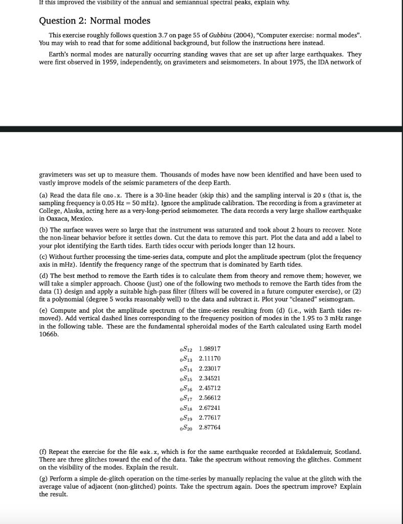
If this improved the visibility of the annual and semiannual spectral peaks, explain why. Question 2: Normal modes This exercise roughly follows question 3.7 on page 55 of Gubbins (2004), "Computer exercise: normal modes". You may wish to read that for some additional background, but follow the instructions here instead. Earth's normal modes are naturally occurring standing waves that are set up after large earthquakes. They were first observed in 1959, independently, on gravimeters and seismometers. In about 1975, the IDA network of gravimeters was set up to measure them. Thousands of modes have now been identified and have been used to vastly improve models of the seismic parameters of the deep Earth. (a) Read the data file cmo.x. There is a 30-line header (skip this) and the sampling interval is 20 s (that is, the sampling frequency is 0.05 Hz = 50 mHz). Ignore the amplitude calibration. The recording is from a gravimeter at College, Alaska, acting here as a very long period seismometer. The data records a very large shallow earthquake in Oaxaca, Mexico. (b) The surface waves were so large that the instrument was saturated and took about 2 hours to recover. Note the non-linear behavior before it settles down. Cut the data to remove this part. Plot the data and add a label to your plot identifying the Earth tides. Earth tides occur with periods longer than 12 hours. (c) Without further processing the time-series data, compute and plot the amplitude spectrum (plot the frequency axis in mHz). Identify the frequency range of the spectrum that dominated by Earth tides. (d) The best method to remove the Earth tides is to calculate them from theory and remove them; however, we will take a simpler approach. Choose (just) one of the following two methods to remove the Earth tides from the data (1) design and apply a suitable high-pass filter (filters will be covered in a future computer exercise), or (2) fit a polynomial (degree 5 works reasonably well) to the data and subtract it. Plot your "cleaned" seismogram. (e) Compute and plot the amplitude spectrum of the time-series resulting from (d) (i.e., with Earth tides re- moved). Add vertical dashed lines corresponding to the frequency position of modes in the 1.95 to 3 mHz range in the following table. These are the fundamental spheroidal modes of the Earth calculated using Earth model 1066b. OS12 1.98917 0913 2.11170 S4 2.23017 Sus 2.34521 S16 2.45712 0917 2.56612 S18 2.67241 S19 2.77617 S20 2.87764 (f) Repeat the exercise for the file esk.x, which is for the same earthquake recorded at Eskdalemuir, Scotland. There are three glitches toward the end of the data. Take the spectrum without removing the glitches. Comment on the visibility of the modes. Explain the result. (g) Perform a simple de-glitch operation on the time-series by manually replacing the value at the glitch with the average value of adjacent (non-glitched) points. Take the spectrum again. Does the spectrum improve? Explain the result. If this improved the visibility of the annual and semiannual spectral peaks, explain why. Question 2: Normal modes This exercise roughly follows question 3.7 on page 55 of Gubbins (2004), "Computer exercise: normal modes". You may wish to read that for some additional background, but follow the instructions here instead. Earth's normal modes are naturally occurring standing waves that are set up after large earthquakes. They were first observed in 1959, independently, on gravimeters and seismometers. In about 1975, the IDA network of gravimeters was set up to measure them. Thousands of modes have now been identified and have been used to vastly improve models of the seismic parameters of the deep Earth. (a) Read the data file cmo.x. There is a 30-line header (skip this) and the sampling interval is 20 s (that is, the sampling frequency is 0.05 Hz = 50 mHz). Ignore the amplitude calibration. The recording is from a gravimeter at College, Alaska, acting here as a very long period seismometer. The data records a very large shallow earthquake in Oaxaca, Mexico. (b) The surface waves were so large that the instrument was saturated and took about 2 hours to recover. Note the non-linear behavior before it settles down. Cut the data to remove this part. Plot the data and add a label to your plot identifying the Earth tides. Earth tides occur with periods longer than 12 hours. (c) Without further processing the time-series data, compute and plot the amplitude spectrum (plot the frequency axis in mHz). Identify the frequency range of the spectrum that dominated by Earth tides. (d) The best method to remove the Earth tides is to calculate them from theory and remove them; however, we will take a simpler approach. Choose (just) one of the following two methods to remove the Earth tides from the data (1) design and apply a suitable high-pass filter (filters will be covered in a future computer exercise), or (2) fit a polynomial (degree 5 works reasonably well) to the data and subtract it. Plot your "cleaned" seismogram. (e) Compute and plot the amplitude spectrum of the time-series resulting from (d) (i.e., with Earth tides re- moved). Add vertical dashed lines corresponding to the frequency position of modes in the 1.95 to 3 mHz range in the following table. These are the fundamental spheroidal modes of the Earth calculated using Earth model 1066b. OS12 1.98917 0913 2.11170 S4 2.23017 Sus 2.34521 S16 2.45712 0917 2.56612 S18 2.67241 S19 2.77617 S20 2.87764 (f) Repeat the exercise for the file esk.x, which is for the same earthquake recorded at Eskdalemuir, Scotland. There are three glitches toward the end of the data. Take the spectrum without removing the glitches. Comment on the visibility of the modes. Explain the result. (g) Perform a simple de-glitch operation on the time-series by manually replacing the value at the glitch with the average value of adjacent (non-glitched) points. Take the spectrum again. Does the spectrum improve? Explain the result


