I'm having such a hard time figuring out how to complete this excel workbook. Hoping to get a detailed step-by-step guide on how to complete steps 2-15. Thanks!
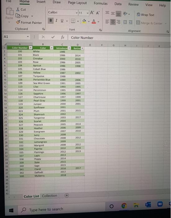
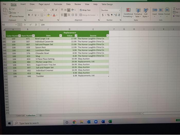
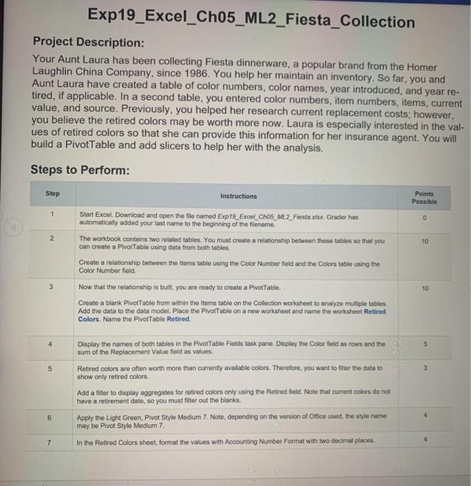
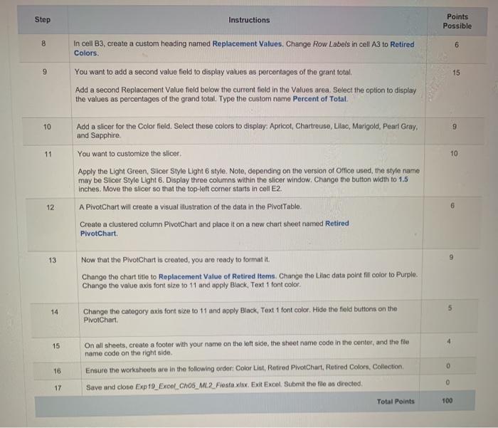
File Home Insert Draw Page Layout Formulas Data Review View Help Xcut In Copy Calibri 11-AA 2 Wrap Text V Paste BIO Format Painter A Merge & Cenfor Clipboard Font Alignment A1 Color Number E H Retire Color White Black Cinnabar 1 2 2 4 5 5 7 8 9 Introduce 1985 1986 2000 1986 Rose 2014 2010 2005 1998 1986 2003 Color Number 100 101 102 103 104 105 106 107 108 109 113 114 116 117 118 119 1986 1987 1988 1989 1991 1993 1995 1996 1997 2006 2005 1995 2008 1997 2001 2001 320 2015 2017 10 11 12 13 14 15 16 17 18 19 20 21 22 23 24 25 26 27 28 29 30 31 32 33 34 35 36 37 38 39 Apricot Cobalt Blue Yellow Turquoise Periwinkle Blue Sea Mist Green Lilac Persimmon Sapphire Chartreuse Pearl Gray Juniper Sunflower Plum Shamrock Tangerine Scarlet Peacock Heather Evergreen Ivory Chocolate Lemongrass Marigold Paprika Flamingo Lapis Poppy Slate Sage Claret Daffodil Mulberry 2000 2001 2001 2002 2003 2004 2005 2006 2007 2008 2008 2009 2008 323 324 325 326 327 328 329 330 331 332 333 334 335 337 338 339 340 341 342 500 2014 2009 2010 2012 2010 2012 2016 2013 2012 2013 2014 2015 2015 2016 2017 2018 2017 10 41 12 Color List Collection Type here to search File Draw Page Layout Formulas Data Review View Help Table Design Auto Number Home Insert Xcut 3 Format Painter Cicboard Calibri AA == 19 Wrap Text BLUA.A. E Meryear Center Fort Alignment $ - % 841 Insert Delete format Conditional Formatas Cell Formatting Table Style Number AZ Jx 104 A G H . 1 Color Numb 144 100 345 100 46 100 100 348 100 349 100 350 100 351 106 352 10G 353 106 106 355 106 356 106 357 106 Item Numb 471 587 497 439 465 $76 453 830 484 121 492 492 453 446 Item Bowl Large 19 Individual Casserole Salt and pepper Set Spoon Rest Luncheon Plate Chowder Bowl Mug 5 Piece Place Setting Pitcher Large Disc SugarCream Tray Set Salt and pepper Set Individual Creamer Mug Tumbler Replacement Value Source 17.99 The Homer Laughlin China Co. 15.99 The Homer Laughlin China Co. 15.99 The Homer Laughlin China Co. 12.99 The Homer Laughlin China Co. 9.99 The Homer Laughlin China Co. 8.99 The Homer Laughlin China Co. 8.49 The Homer Laughlin China Co. 33.99 Ebay Auction 29.99 Replacements, Ltd 26.99 Ebay Auction 19.95 thay Auction 16.99 Ebay Auction 9.09 thay Auction 6.99 Replacements, Ltd 380 361 362 06) 364 165 166 368 369 TO Color List Collection 100 G . Type here to search Exp19_Excel_Ch05_ML2_Fiesta_Collection Project Description: Your Aunt Laura has been collecting Fiesta dinnerware, a popular brand from the Homer Laughlin China Company, since 1986. You help her maintain an inventory. So far, you and Aunt Laura have created a table of color numbers, color names, year introduced, and year re- tired, if applicable. In a second table, you entered color numbers, item numbers, items, current value, and source. Previously, you helped her research current replacement costs; however, you believe the retired colors may be worth more now. Laura is especially interested in the val- ues of retired colors so that she can provide this information for her insurance agent. You will build a PivotTable and add slicers to help her with the analysis. Steps to Perform: Step Points Possible 1 2 10 Instructions Start Excel. Download and open the file named Exp19_Excel_Cho5_ML2 Fiesta xlsx. Grader has automatically added your last name to the beginning of the filename. The workbook contains two related tables. You must create a relationship between these tables so that you can create a Pivot Table using data from both tables. Create a relationship between the items table using the Color Number field and the Colors table using the Color Number field Now that the relationship is built, you are ready to creato a Pivottable. Creato a blank Pivot Table from within the items tablo on the Collection worksheet to analyze multiple tables. Add the data to the data model. Place the Pivot Table on a new worksheet and name the worksheet Retired Colors. Name the Pivot Table Retired. 3 10 4 5 5 3 Display the names of both tables in the Pivottable Fields task pano. Display the Color Seld as rows and the sum of the Replacement Value field as values. Retired colors are often worth more than currently available colors. Therefore, you want to filter the data to show only retired colors Add a filter to display aggregates for retired colors only using the Retired field. Note that current colors do not have a retirement date, so you must filter out the blanks. Apply the Light Green, Pivot Style Medium 7. Noto, depending on the version of Ollice used the style name may be Pivot Style Mediurn 7. In the Retired Colors sheet, format the values with Accounting Number Format with two decimal places 6 4 7 Step Instructions Points Possible 8 In cell B3, create a custom heading named Replacement Values. Change Row Labels in cell A3 to Retired 6 Colors, 9 15 You want to add a second value field to display values as percentages of the grant total Add a second Replacement Value field below the current field in the Values area. Select the option to display the values as percentages of the grand total. Type the custom name Percent of Total 10 9 11 10 Add a slicer for the Color field. Select those colors to display, Apricot, Chartreuse, Lilac, Marigold, Pearl Gray and Sapphire You want to customize the slicer. Apply the Light Green, Slicer Style Light 6 style. Note, depending on the version of Office used the style name may be Slicer Style Light 6. Display three columns within the slicer window. Change the button width to 1.5 inches. Move the slicer so that the top-left corner starts in cell E2. A PivotChart will create a visual illustration of the data in the Pivot Table Create a clustered column PivotChart and place it on a new chart sheet named Retired PivotChart. 12 6 9 13 Now that the PivotChart is created, you are ready to format it. Change the chart title to Replacement Value of Retired Items Change the Lilac data point fill color to Purple. Change the value axis font size to 11 and apply Black, Text 1 font color. 14 Change the category axis font size to 11 and apply Black, Text 1 font color. Hide the fold buttons on the PivotChart 15 On all sheets, create a footer with your name on the left side, the sheet name code in the center, and the file name code on the right side. Ensure the workshoots are in the following order: Color List, Retired PivotChart, Retired Colors, Collection, Save and close Exp19_Excel Cho5_ML2 Fiesta xnx. Exit Excel Submit the file as directed 0 16 17 Total Points 100