im not sure how to do any of this but the first and second step
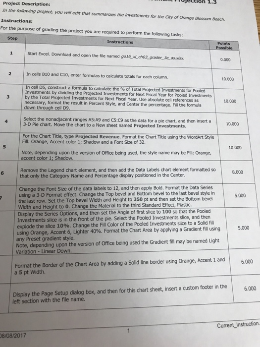
Tujettion 1.3 Project Description: In the folowing project, you wW edit that summarizes the investments for the City of Orange Blossom Beach. For the purpose of grading the project you are required to perform the following tasks: Step Instructions Points 1 Start Excel. Download and open the file named go16 xLchos grader 3e.as.xlsx. 0.000 In cells B10 and C10, enter formulas to calculate totals for each column. 10.000 In cell D5, construct a formula to calculate the % of Total Projected Investments for Investments by dividing the Projected by the Total Projected Investments for Next Fiscal Year. Use absolute cell references as nvestments for Next Fiscal Year for Pooled 3 necessary, format the result in Percent Style, and Center the percentage. Fill the formula 10.000 down through cell D9 Select the nonadjacent ranges AS:A9 and C5:C9 as the data for a pie chart, and then insert a 3-D Pie chart. Move the chart to a New sheet named Projected Investments. 10.000 For the Chart Title, type Projected Revenue. Format the Chart Title using the WordArt Style Fill: Orange, Accent color 1; Shadow and a Font Size of 32. 10.000 Note, depending upon the version of Office being used, the style name may be Fill: Orange, accent color l Shadow. Remove the Legend chart element, and then add the Data Labels chart element formatted so that only the Category Name and Percentage display positioned in the Center. 6 Change the Font Size of the data labels to 12, and then apply Bold. Format the Data Series using a 3-D Format effect. Change the Top bevel and Bottom bevel to the last bevel style in the last row. Set the Top bevel Width and Height to 350 pt and then set the Bottom bevel Width and Height to O. Change the Material to the third Standard Effect, Plastic. Display the Series Options, and then set the Angle of first slice to 100 so that the Pooled Investments slice is in the front of the pie. Select the Pooled Investments slice, and then explode the slice 10%. Change the Fill Color of the Pooled Investments slice to a solid fill using Orange, Accent 6, Lighter 40%. Format the Chart Area by applying a Gradient fill using any Preset gradient style Note, depending upon the version of Office being used the Gradient fill may be named Light Variation-Linear Down 5.000 Format the Border of the Chart Area by adding a Solid line border using Orange, Accent 1 and a 5 pt Width. 6.000 Display the Page Setup dialog box, and then for this chart sheet, insert a custom footer in the6.000 left section with the file name. Current_Instruction. 8/08/2017 Tujettion 1.3 Project Description: In the folowing project, you wW edit that summarizes the investments for the City of Orange Blossom Beach. For the purpose of grading the project you are required to perform the following tasks: Step Instructions Points 1 Start Excel. Download and open the file named go16 xLchos grader 3e.as.xlsx. 0.000 In cells B10 and C10, enter formulas to calculate totals for each column. 10.000 In cell D5, construct a formula to calculate the % of Total Projected Investments for Investments by dividing the Projected by the Total Projected Investments for Next Fiscal Year. Use absolute cell references as nvestments for Next Fiscal Year for Pooled 3 necessary, format the result in Percent Style, and Center the percentage. Fill the formula 10.000 down through cell D9 Select the nonadjacent ranges AS:A9 and C5:C9 as the data for a pie chart, and then insert a 3-D Pie chart. Move the chart to a New sheet named Projected Investments. 10.000 For the Chart Title, type Projected Revenue. Format the Chart Title using the WordArt Style Fill: Orange, Accent color 1; Shadow and a Font Size of 32. 10.000 Note, depending upon the version of Office being used, the style name may be Fill: Orange, accent color l Shadow. Remove the Legend chart element, and then add the Data Labels chart element formatted so that only the Category Name and Percentage display positioned in the Center. 6 Change the Font Size of the data labels to 12, and then apply Bold. Format the Data Series using a 3-D Format effect. Change the Top bevel and Bottom bevel to the last bevel style in the last row. Set the Top bevel Width and Height to 350 pt and then set the Bottom bevel Width and Height to O. Change the Material to the third Standard Effect, Plastic. Display the Series Options, and then set the Angle of first slice to 100 so that the Pooled Investments slice is in the front of the pie. Select the Pooled Investments slice, and then explode the slice 10%. Change the Fill Color of the Pooled Investments slice to a solid fill using Orange, Accent 6, Lighter 40%. Format the Chart Area by applying a Gradient fill using any Preset gradient style Note, depending upon the version of Office being used the Gradient fill may be named Light Variation-Linear Down 5.000 Format the Border of the Chart Area by adding a Solid line border using Orange, Accent 1 and a 5 pt Width. 6.000 Display the Page Setup dialog box, and then for this chart sheet, insert a custom footer in the6.000 left section with the file name. Current_Instruction. 8/08/2017