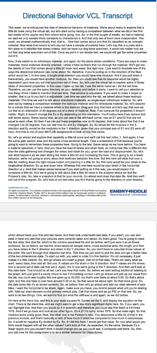
Image transcription text

Directional Behavior VCL Transcript This week, we've introduced the idea of directional behavior of
materials. We're about ready to explore that a little bit more using the virtual lab, but let's start out by having
a comparison between what we did in the first two weeks of the course and then where we're ... 

 

Image transcription text

% The purpose of this code is to % (1) plot the material properties as a function of primary axis direction %
"start by closing all existing windows and plots that are open close all; clear all; % Use the properties
below to get started. They are taken directly from Figure 2. 11. This way you can compare your ... 

Image transcription text

9696 6969696636966969696969%%696%*%% Important Note xx696936
6463696369696969696969696%% " Do not delete any part of this script. It is ok to add to it and
comment * out material that is not required, but do not delete anything * Insert Student Name * ... 

Image transcription text

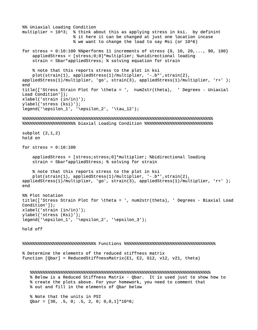
%% Uniaxial Loading Condition multiplier = 1043; % think about this as applying stress in ksi. by definint % it
here it can be changed at just one location incase % we want to change the load to say Msi (or 1046) for
stress = 0:10:100 %%performs 11 increments of stress {0, 10, 20, . .., 90, 100} appliedStress = [s... 

Image transcription text

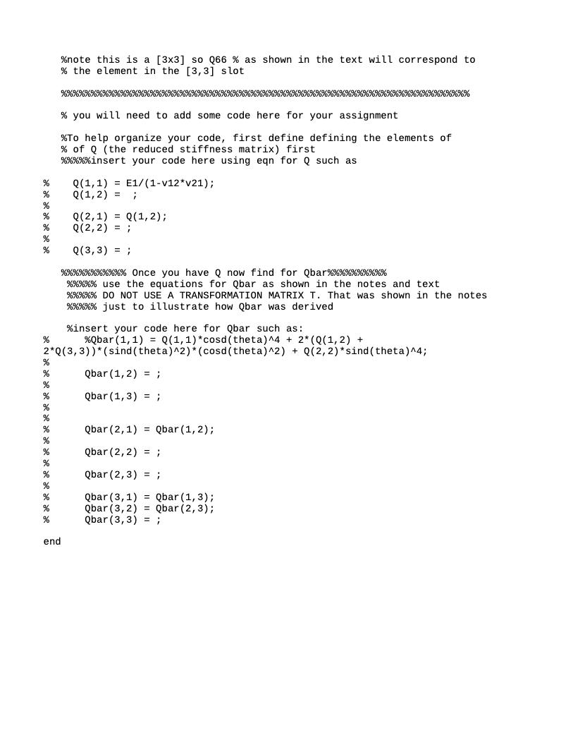
"note this is a [3x3] so Q66 % as shown in the text will correspond to % the element in the [3, 3] slot %
you will need to add some code here for your assignment "To help organize your code, first define
defining the elements of % of Q ( the reduced stiffness matrix) first *%%%%%insert your code ... 

Image transcription text

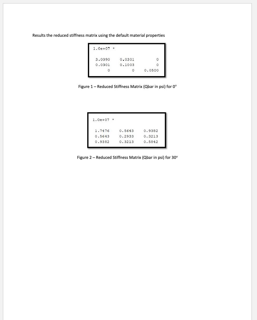
Results the reduced stiffness matrix using the default material properties 1 .0e+0'? - 3.0030 0.0301 0
0.030.]. 0.1003 0 0 0 0.0500 Figure l ? Reduced Stiffness Matrix [?ber in psi} for 0° Figure 2 ? Reduced
Stiffness Matrix [Ctbar in psi} for 30"
 

Directional Behavior VCL Transcript This week, we've introduced the idea of directional behavior of materials. We're about ready to explore that a little bit more using the virtual lab, but let's start out by having a comparison between what we did in the first two weeks of the course and then where we're going now. So, in the first couple of weeks, we had a material. we said we only needed three constants to characterize it. And that only two of them were independent. This week, we showed mathematically that, that is... How that comes about and that it's classified as an isotropic material. Now what that means is let's say we have a sample of material here. Let's say this is a plate and a thin plate so it satisfies that stress criteria. And we have our dog bone specimen. It would not matter how we cut that dog bone specimen out of that. Once we put it in our tensile test, we would still get the same properties out of it. Now, if we switch to an orthotropic material, and again, for the plane stress conditions. There are ways to make materials, these materials directly oriented. I show it here as fibers that run through the material. We'll get into the details of how that comes about a little bit more next week. But right now, I just want to illustrate one of the ways the directional behavior can come about. So, therefore, if you're pulling on in the direction of the fiber, which would be 1, in this case, a longitudinal direction you would have one modulus. And if you pull down it transversely, you would have another modulus. So, then you could see that its response would be highly dependent upon how you cut that specimen out of there. So, let's use the virtual lab to explore some of those ideas of directional properties. In this case, I open up the lab, I use the same name as I did the last time. Therefore, we can use the same directory on your desktop and before it starts, I want to call your attention to one thing I think I failed to mention that last time. That window is adjustable. If you want to make it larger or smaller, that is up to you but it is adjustable. Last time we went into the lab, we talked about these isotropic materials. This time we want to talk about directional materials, so single-layer orthotropic material. So, let's start out by making a comparison between the isotropic material and the directional material. So, let's assume for a minute that we have a material which is like titanium. Drag and drop that here and let's say that now we cut that at an orientation of 45 degrees out of a piece of material. Now, if we compute the properties it doesn't matter. Right, it doesn't change the Ex or Ey depending on the orientation. You'll notice here if we replace that with boron epoxy, Boron epoxy now, as you can see in the left-hand corner, has an E1 and E2 that are not equal to each other. So then if we can put these properties now at 45 degrees, that looks about like that if we changed it to 30 degrees. You can see how Ex and Ey changed. So, Ex would be the modulus in the X direction and Ey would be the modulars in the Y direction, given that your principal axis of E1 and E2 were off here. And that is one of your MATLAB assignments to look at how that varies. So, let's go ahead and explore that capability a little bit more and we'll call this test ortho_1. And again, it has the same gate section area and the same cross-sectional length. Take a screenshot of that because you're going to want to remember these properties here. Going to the test. Same setup as we have before. You have a material specimen in here. And you have the load of stress and strain here, so notice how this is different this time the data gathering tool changes the stress and strain for you, given the load and displacement. So, let's see what happens as we start sliding the slider a little bit and increasing the load. This is going to be a linear behavior; we're not going to worry about that nonlinear behavior this time. But this here will slide that over a little bit, holding down the right mouse button and panning it a little bit. So, this here would be your strain in the longitudinal direction. So up and down here. Whereas this one here would be your strain in the horizontal direction or y. And that makes sense because if you start pulling on it this way, you would expect it to compress a little bit. And we're going to talk about that a little bit more in the analysis where we find the Poisson's ratio. So, take a snapshot of that for your records. Go ahead and close that data file. And then we'll exit out of the program. So, let's look at our test data, you find that by going to the directory on your desktop, worldwide.erau.edu All rights are reserved. The material contained herein is the copyright property of Embry-Riddle Aeronautical system, or transmitted in any form, electronic, mechanical, photocopying, recording or otherwise without the University, Daytona Beach, Florida, 32114. No part of this material may be reproduced, stored in a retrieval prior written consent of the University. EMBRY-RIDDLE Aeronautical University which should have your first and last name. And then look underneath test data. If you aren't, you can also peek in here and see that your pictures were correctly taken and saved. So that's good. You're going to need the test data. See that file, which is the comma-separated file and as before, we'll just save it as an Excel workbook. So as before, we had the cross-sectional sample name, cross-sectional area, the length, and then you have stress in the X direction and strain in the Y direction. So, you don't have to calculate those values at this point. We went through that objective last time. This time we just want to plot the data and get a better idea of the two-dimensional state. To start out with, you want to order it in this fashion. It's not necessary, it just makes it a little cleaner. So, let's go ahead and insert a graph. Get rid of that data. That's not really what we want, select data, then add all. Set one. X values are the strain in the X direction. And Y values are the stress. And a second set of data call that set 2. Again, the X now we're going to the Y direction. And then we'll look at this data here. That should be all set. Let's see how that looks. So, before we start adding additional labeling to the graph, let's just give it a sanity check to see if it's looking correct. Let's go ahead and pull up our visual from the lab, you could see roughly this one goes up to 20,000, but that's over there at about 0.05. So that's about right, and this one here is over here around 0.02 or so. So that would be about right. So that looks good. So, the data looks like it's all stored correctly. So, as before, then let's go ahead and add our chart element of axis titles. I want the horizontal to be strain. Again, make sure you have, you remind people what unit you're dealing with. Add our chart element on the primary vertical axis. Call that stress and we go PSI on that one. So, we want to do two things. One, we want to find out what the stiffness is and again, as we did before. I'm here at the trend line, and this is your least squares fit. Center set the 0, and display the equation on the chart. There is the trend line, and we might want to get a few more significant digits here. So, if you want, you can highlight that. And then you would do it in scientific and therefore you could see that that's a 4.6 times 10^6. And if we go back and look at our other figure, it's 4.27 I'm sorry, times 10^6. So that looks right. So that modulus looks pretty good. Now, the other one is the Poisson's ratio. You discovered a little bit of that in the previous module, and that's basically a ratio of how much it stretches compared to how much it compresses. So, it would be negative Ey divided by Ex. So, if I did this here, I would get that value. So now what would you think would happen with all the other values? Let's look at that. As expected, it's the same. Because it's a linear region and you wouldn't think it would change and as you could see, it compares well there. So, then your job now for this assignment is to do a similar behavior for Glass Epoxy.