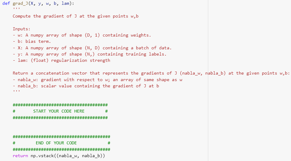
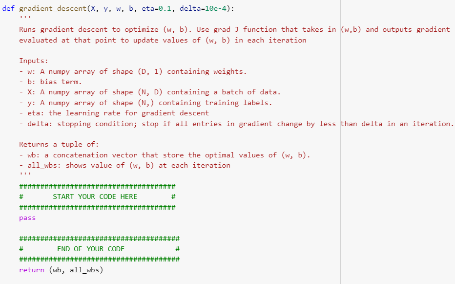
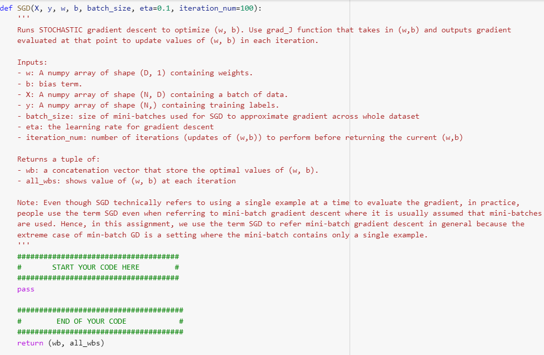
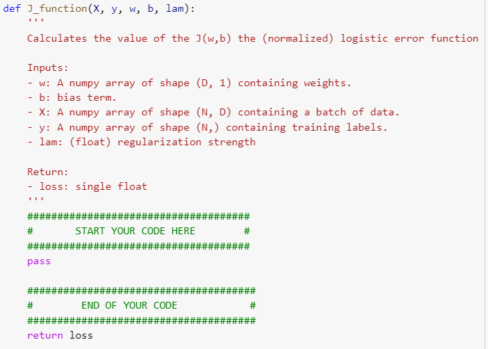
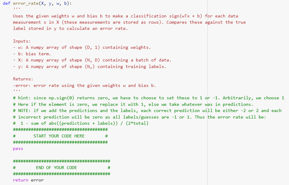
Implement gradient descent with an initial iterate of all zeros. Using the gradients wJ(w,b),bJ(w,b), which are derived in Question 4 of the writing part, complete the following functions, i.e., grad_J,J_function,error_rate,gradient_descent, and SGD.

Try several values of learning rates to find one that appears to make convergence on the training set as fast as possible. Run until you feel you are near to convergence.

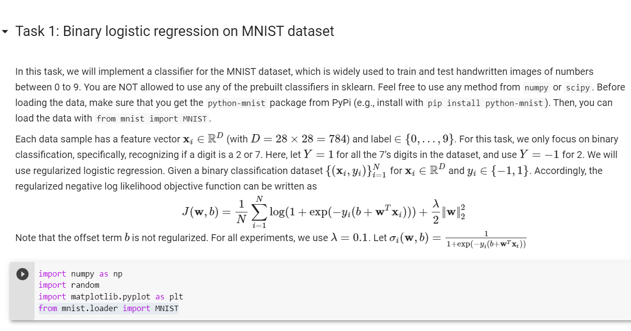
Task 1: Binary logistic regression on MNIST dataset In this task, we will implement a classifier for the MNIST dataset, which is widely used to train and test handwritten images of numbers between 0 to 9. You are NOT allowed to use any of the prebuilt classifiers in sklearn. Feel free to use any method from numpy or scipy. Before loading the data, make sure that you get the python-mnist package from PyPi (e.g., install with pip install python-mnist). Then, you can load the data with from mnist import MNIST. Each data sample has a feature vector Xi E RD (with D = 28 x 28 = 784) and label {0,...,9}. For this task, we only focus on binary classification, specifically, recognizing if a digit is a 2 or 7. Here, let Y = 1 for all the 7's digits in the dataset, and use Y = -1 for 2. We will use regularized logistic regression. Given a binary classification dataset {(Xi, yi)}N1 for xi RD and yi {-1,1}. Accordingly, the regularized negative log likelihood objective function can be written as N 1 J(w,b) + N 2 Note that the offset term b is not regularized. For all experiments, we use l = 0.1. Let oi(w,5) = 1+exp(-yi(b+w+'x;)) 1 import numpy as np import random import matplotlib.pyplot as plt from mnist.loader import MNIST def grad_](x, y, w, b, lam): Compute the gradient of I at the given points w,b Inputs: - W: A numpy array of shape (D, 1) containing weights. - b: bias term. - X: A numpy array of shape (N, D) containing a batch of data. - y: A numpy array of shape (N,) containing training labels. - lam: (float) regularization strength Return a concatenation vector that represents the gradients of i (nabla_w, nabla_b) at the given points w,b: - nabla_w: gradient with respect to w; an array of same shape as w nabla_b: scalar value containing the gradient of ] at b ##################################### # START YOUR CODE HERE # ##################################### ###################################### # END OF YOUR CODE # ###################################### return np.vstack((nabla_w, nabla_b)) def J_function(x, y, w, b, lam): Calculates the value of the J(w,b) the (normalized) logistic error function Inputs: w: A numpy array of shape (D, 1) containing weights. - b: bias term. X: A numpy array of shape (N, D) containing a batch of data. y: A numpy array of shape (N,) containing training labels. - lam: (float) regularization strength Return: - loss: single float # START YOUR CODE HERE pass F # # # ### END OF YOUR CODE FF # # FIF 11 # ELLE HE # return loss def error_rate(x, y, w, b): Uses the given weights w and bias b to make a classification sign (WTx + b) for each data measurement x in X (these measurements are stored as rows). Compares these against the true label stored in y to calculate an error rate. Inputs: - w: A numpy array of shape (D, 1) containing weights. - b: bias term. - X: A numpy array of shape (N, D) containing a batch of data. - y: A numpy array of shape (N,) containing training labels. Returns: -error: error rate using the given weights w and bias b. # hint: since np.sign () returns zero, we have to choose to set these to 1 or -1. Arbitrarily, we choose 1 # Here if the element is zero, we replace it with 1, else we take whatever was in predictions. # NOTE: if we add the predictions and the labels, each correct prediction will be either -2 or 2 and each # incorrect prediction will be zero as all labels/guesses are -1 or 1. Thus the error rate will be: # 1 - sum of abs((predictions + labels)) / (2*total) ##################################### # START YOUR CODE HERE # pass ###################################### # END OF YOUR CODE # ###################################### return error def gradient_descent(X, Y, W, b, eta=0.1, delta=10e-4): Runs gradient descent to optimize (w, b). Use grad_j function that takes in (w,b) and outputs gradient evaluated at that point to update values of (w, b) in each iteration Inputs: W: A numpy array of shape (D, 1) containing weights. b: bias term. X: A numpy array of shape (N, D) containing a batch of data. y: A numpy array of shape (N,) containing training labels. - eta: the learning rate for gradient descent - delta: stopping condition; stop if all entries in gradient change by less than delta in an iteration. Returns a tuple of: - wb: a concatenation vector that store the optimal values of (w, b). - all_wbs: shows value of (w, b) at each iteration # START YOUR CODE HERE pass ### END OF YOUR CODE # # return (wb, all_wbs) def SGD(x, y, w, b, batch_size, eta=0.1, iteration_num=100): Runs STOCHASTIC gradient descent to optimize (w, b). Use grad_j function that takes in (w,b) and outputs gradient evaluated at that point to update values of (w, b) in each iteration. Inputs: - W: A numpy array of shape (0, 1) containing weights. - b: bias term. - X: A numpy array of shape (N, D) containing a batch of data. - y: A numpy array of shape (N,) containing training labels. - batch_size: size of mini-batches used for SGD to approximate gradient across whole dataset - eta: the learning rate for gradient descent iteration_num: number of iterations (updates of (w,b)) to perform before returning the current (w,b) Returns a tuple of: - wb: a concatenation vector that store the optimal values of (w, b). - all_wbs: shows value of (w, b) at each iteration Note: Even though SGD technically refers to using a single example at a time to evaluate the gradient, in practice, people use the term SGD even when referring to mini-batch gradient descent where it is usually assumed that mini-batches are used. Hence, in this assignment, we use the term SGD to refer mini-batch gradient descent in general because the extreme case of min-batch GD is a setting where the mini-batch contains only a single example. ##################################### # START YOUR CODE HERE # ############### ################ pass ###################################### # END OF YOUR CODE # ###################################### return (wb, all_wbs) Task 1: Binary logistic regression on MNIST dataset In this task, we will implement a classifier for the MNIST dataset, which is widely used to train and test handwritten images of numbers between 0 to 9. You are NOT allowed to use any of the prebuilt classifiers in sklearn. Feel free to use any method from numpy or scipy. Before loading the data, make sure that you get the python-mnist package from PyPi (e.g., install with pip install python-mnist). Then, you can load the data with from mnist import MNIST. Each data sample has a feature vector Xi E RD (with D = 28 x 28 = 784) and label {0,...,9}. For this task, we only focus on binary classification, specifically, recognizing if a digit is a 2 or 7. Here, let Y = 1 for all the 7's digits in the dataset, and use Y = -1 for 2. We will use regularized logistic regression. Given a binary classification dataset {(Xi, yi)}N1 for xi RD and yi {-1,1}. Accordingly, the regularized negative log likelihood objective function can be written as N 1 J(w,b) + N 2 Note that the offset term b is not regularized. For all experiments, we use l = 0.1. Let oi(w,5) = 1+exp(-yi(b+w+'x;)) 1 import numpy as np import random import matplotlib.pyplot as plt from mnist.loader import MNIST def grad_](x, y, w, b, lam): Compute the gradient of I at the given points w,b Inputs: - W: A numpy array of shape (D, 1) containing weights. - b: bias term. - X: A numpy array of shape (N, D) containing a batch of data. - y: A numpy array of shape (N,) containing training labels. - lam: (float) regularization strength Return a concatenation vector that represents the gradients of i (nabla_w, nabla_b) at the given points w,b: - nabla_w: gradient with respect to w; an array of same shape as w nabla_b: scalar value containing the gradient of ] at b ##################################### # START YOUR CODE HERE # ##################################### ###################################### # END OF YOUR CODE # ###################################### return np.vstack((nabla_w, nabla_b)) def J_function(x, y, w, b, lam): Calculates the value of the J(w,b) the (normalized) logistic error function Inputs: w: A numpy array of shape (D, 1) containing weights. - b: bias term. X: A numpy array of shape (N, D) containing a batch of data. y: A numpy array of shape (N,) containing training labels. - lam: (float) regularization strength Return: - loss: single float # START YOUR CODE HERE pass F # # # ### END OF YOUR CODE FF # # FIF 11 # ELLE HE # return loss def error_rate(x, y, w, b): Uses the given weights w and bias b to make a classification sign (WTx + b) for each data measurement x in X (these measurements are stored as rows). Compares these against the true label stored in y to calculate an error rate. Inputs: - w: A numpy array of shape (D, 1) containing weights. - b: bias term. - X: A numpy array of shape (N, D) containing a batch of data. - y: A numpy array of shape (N,) containing training labels. Returns: -error: error rate using the given weights w and bias b. # hint: since np.sign () returns zero, we have to choose to set these to 1 or -1. Arbitrarily, we choose 1 # Here if the element is zero, we replace it with 1, else we take whatever was in predictions. # NOTE: if we add the predictions and the labels, each correct prediction will be either -2 or 2 and each # incorrect prediction will be zero as all labels/guesses are -1 or 1. Thus the error rate will be: # 1 - sum of abs((predictions + labels)) / (2*total) ##################################### # START YOUR CODE HERE # pass ###################################### # END OF YOUR CODE # ###################################### return error def gradient_descent(X, Y, W, b, eta=0.1, delta=10e-4): Runs gradient descent to optimize (w, b). Use grad_j function that takes in (w,b) and outputs gradient evaluated at that point to update values of (w, b) in each iteration Inputs: W: A numpy array of shape (D, 1) containing weights. b: bias term. X: A numpy array of shape (N, D) containing a batch of data. y: A numpy array of shape (N,) containing training labels. - eta: the learning rate for gradient descent - delta: stopping condition; stop if all entries in gradient change by less than delta in an iteration. Returns a tuple of: - wb: a concatenation vector that store the optimal values of (w, b). - all_wbs: shows value of (w, b) at each iteration # START YOUR CODE HERE pass ### END OF YOUR CODE # # return (wb, all_wbs) def SGD(x, y, w, b, batch_size, eta=0.1, iteration_num=100): Runs STOCHASTIC gradient descent to optimize (w, b). Use grad_j function that takes in (w,b) and outputs gradient evaluated at that point to update values of (w, b) in each iteration. Inputs: - W: A numpy array of shape (0, 1) containing weights. - b: bias term. - X: A numpy array of shape (N, D) containing a batch of data. - y: A numpy array of shape (N,) containing training labels. - batch_size: size of mini-batches used for SGD to approximate gradient across whole dataset - eta: the learning rate for gradient descent iteration_num: number of iterations (updates of (w,b)) to perform before returning the current (w,b) Returns a tuple of: - wb: a concatenation vector that store the optimal values of (w, b). - all_wbs: shows value of (w, b) at each iteration Note: Even though SGD technically refers to using a single example at a time to evaluate the gradient, in practice, people use the term SGD even when referring to mini-batch gradient descent where it is usually assumed that mini-batches are used. Hence, in this assignment, we use the term SGD to refer mini-batch gradient descent in general because the extreme case of min-batch GD is a setting where the mini-batch contains only a single example. ##################################### # START YOUR CODE HERE # ############### ################ pass ###################################### # END OF YOUR CODE # ###################################### return (wb, all_wbs)