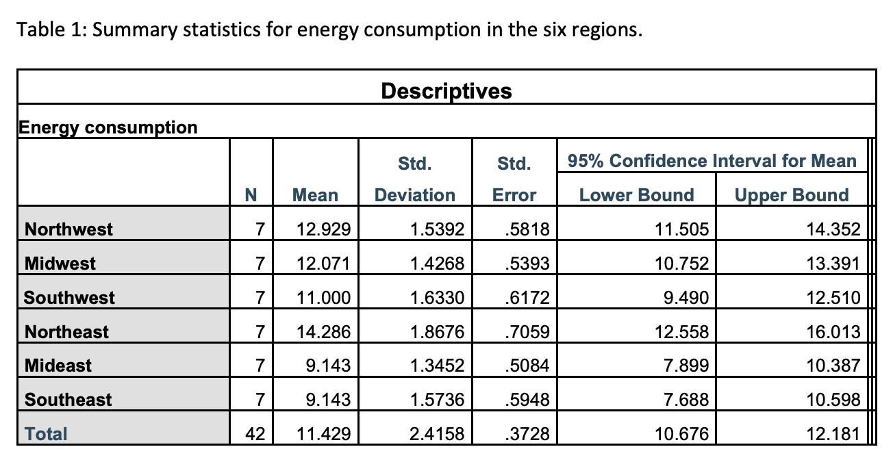
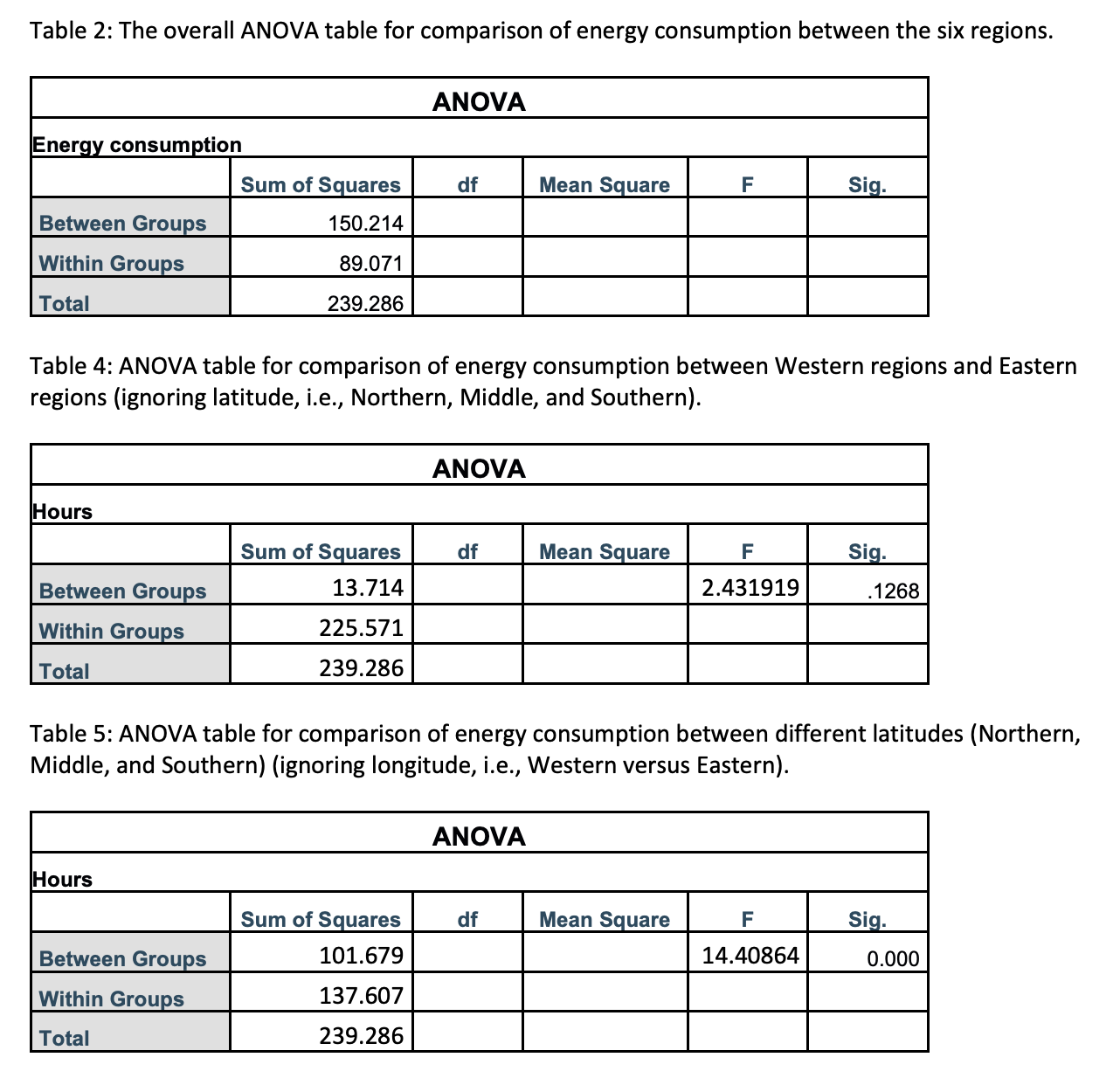
In a certain country, a study was conducted to compare energy consumption (in BTUs) in six different regions (Northwest, Midwest, Southwest, Northeast, Mideast, and Southeast). Assume that all assumptions are met for the required analyses. All relevant information can be found in Tables 1 to 3. Parameters are defined as follows: ?

?_NW = Northwest region ?_MW = Midwest region ?

?_SW = Southwest region ?

?_NE = Northeast region ?

?_ME = Mideast region ?

?_SE = Southeast region

(a) At the 1% significance level, carry out the most appropriate test to determine if there are any significant difference in mean energy consumption among the six regions. SHOW ALL STEPS.

(b) What is the best estimate for the common or pooled standard deviation of the 6 populations?

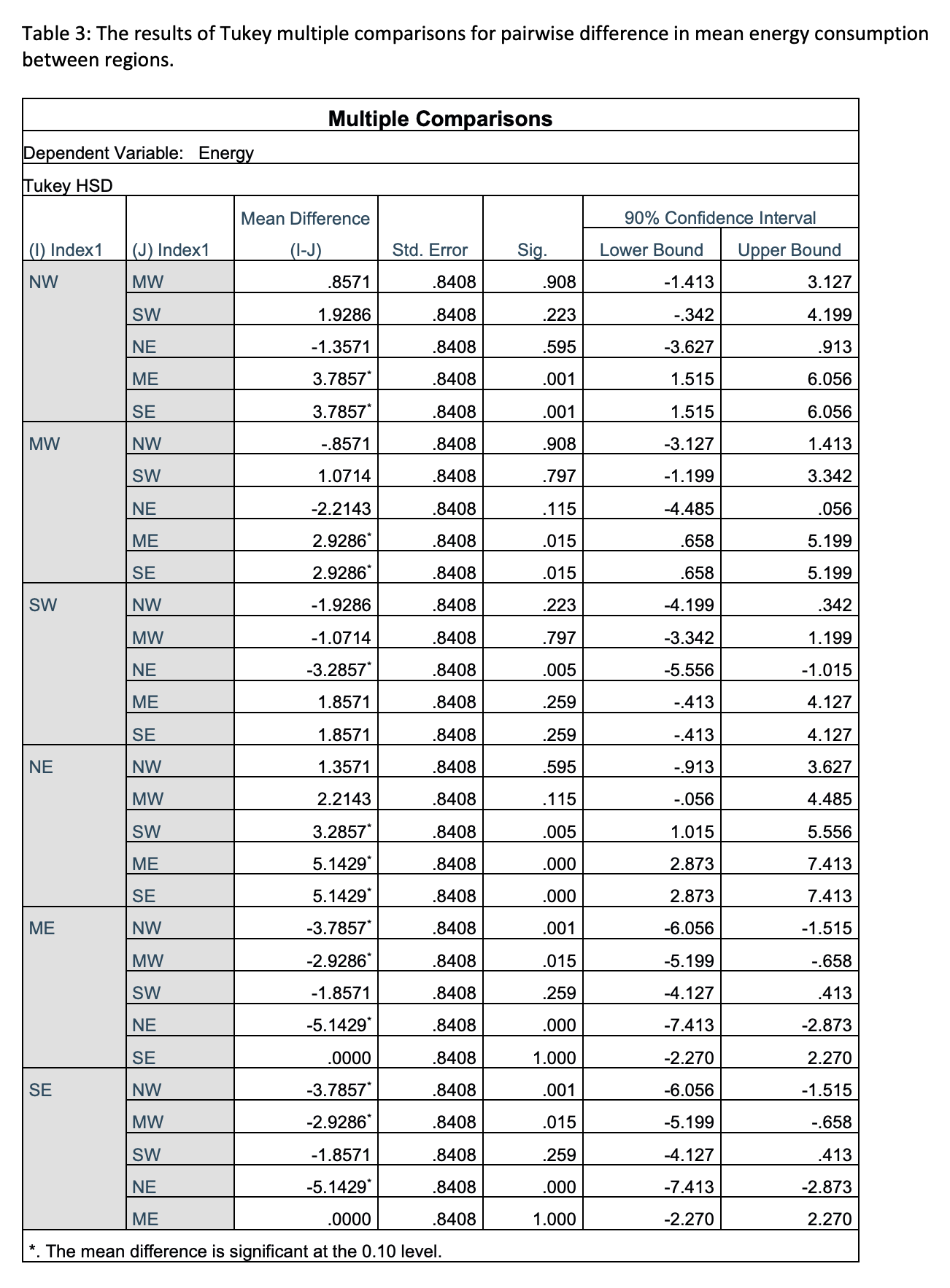
(c) Based on the SPSS output for Tukey's multiple comparisons performed at the 90% confidence level (Table 3), firstly, construct a means comparisons diagram and, secondly, summarize the results in words.

(d) At the 97% confidence level, perform the Bonferroni method of multiple comparisons to determine which pairs of regions have different mean energy consumption. SHOW ALL STEPS, including compilation of the results in a matrix and giving the conclusion both in a means comparisons diagram and in words. Note: You only have to calculate the margin of error once since sample sizes are equal for all groups.

(e) Compare the means comparisons diagrams you constructed in parts (c) and (d). Do they show the same results? If they show different results, explain the reasons for the difference. If they show the same results, state whether they must show the same results, or whether they could have shown different results, explaining the reasons for potential differences.

(f) Develop a linear combination (contrast) to test the hypothesis that there is a difference in energy consumption between the Northwest and Midwest regions (combined) in comparison with the Northeast and Mideast regions (combined). Then, test this contrast at the 1% significance level. SHOW ALL STEPS of the hypothesis test.

(g) Develop a linear combination (contrast) to test the hypothesis that there is a difference in energy consumption between the Northwest region and the combined Eastern regions (i.e., Northeast, Mideast, and Southeast combined). Then, test this contrast at the 1% significance level. SHOW ALL STEPS of the hypothesis test.

Table 2: The overall ANOVA table for comparison of energy consumption between the six regions. ANOVA Energy consumption Sum of Squares df Mean Square F Sig Between Groups 150.214 Within Groups 89.071 Total 239.286 Table 4: ANOVA table for comparison of energy consumption between Western regions and Eastern regions (ignoring latitude, i.e., Northern, Middle, and Southern). ANOVA Hours Sum of Squares df Mean Square F Sig Between Groups 13.714 2.431919 1268 Within Groups 225.571 Total 239.286 Table 5: ANOVA table for comparison of energy consumption between different latitudes (Northern, Middle, and Southern) (ignoring longitude, i.e., Western versus Eastern). ANOVA Hours Sum of Squares df Mean Square F Sig Between Groups 101.679 14.40864 0.000 Within Groups 137.607 Total 239.286Table 1: Summary statistics for energy consumption in the six regions. Descriptives Energy consumption Std. Std. 95% Confidence Interval for Mean N Mean Deviation Error Lower Bound Upper Bound Northwest 7 12.929 1.5392 5818 11.505 14.352 Midwest 7 12.071 1.4268 5393 10.752 13.391 Southwest 7 11.000 1.6330 6172 9.490 12.510 Northeast 7 14.286 1.8676 7059 12.558 16.013 Mideast 7 9.143 1.3452 .5084 7.899 10.387 Southeast 7 9.143 1.5736 5948 7.688 10.598 Total 42 11.429 2.4158 3728 10.676 12.181Table 2: The overall ANOVA table for comparison of energy consumption between the six regions. ANOVA Energy consumption Sum of Squares df Mean Square F Sig. Between Groups 150.214 Within Groups 89.071 Total 239.286Table 3: The results of Tukey multiple comparisons for pairwise difference in mean energy consumption between regions. Multiple Comparisons Dependent Variable: Energy Tukey HSD Mean Difference 90% Confidence Interval (1) Index 1 (J) Index 1 ( 1-J) Std. Error Sig. Lower Bound Upper Bound NW .8571 8408 908 -1.413 3.127 SW 1.9286 8408 223 .342 4. 199 NE -1.3571 8408 595 -3.627 913 ME 3.7857 8408 001 1.515 6.056 SE 3.7857* 8408 001 1.515 6.056 MW NW .8571 .8408 908 -3.127 1.413 SW 1.0714 840 797 -1.19 3.342 NE -2.2143 8408 115 -4.485 56 ME 2.9286* 8408 015 658 5.199 SE 2.9286 8408 015 658 5. 199 SW VW -1.9286 .8408 223 -4.199 342 MW -1.0714 8408 797 -3.342 1.199 NE 3.2857 8408 05 -5.556 -1.015 ME 1.8571 8408 259 .413 4.127 SE 1.8571 8408 259 .413 4.127 NE VW 1.3571 .8408 595 .913 3.627 MW 2.2143 8408 115 .056 4.485 SW 3.2857' 8408 005 1.015 5.556 ME 5.1429* 8408 000 2.873 7.413 SE 5.1429 8408 .000 2.873 7.413 ME NW -3.7857 8408 001 -6.056 -1.515 MW -2.9286 8408 015 -5.199 ..658 SW -1.8571 8408 259 -4.127 413 NE -5.1429* 8408 000 -7.413 -2.873 SE .0000 .8408 1.000 -2.270 2.270 SE VW -3.7857 8408 001 -6.056 -1.515 MW -2.9286* 8408 015 -5.199 .658 SW 1.8571 8408 259 -4.127 413 NE -5.1429* 8408 000 -7.413 2.873 ME .0000 .8408 1.000 -2.270 2.270 *. The mean difference is significant at the 0.10 level