In Python3
Don't use preprocessing from sklearn
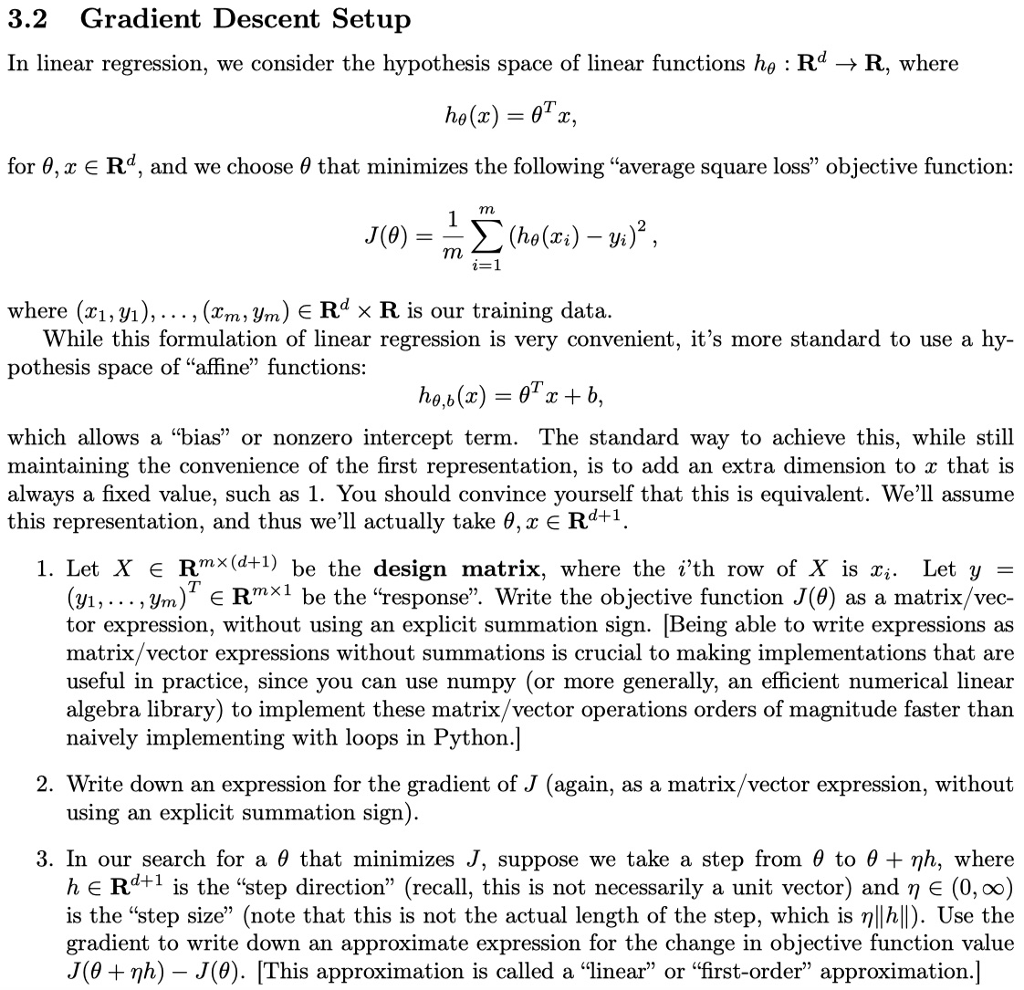
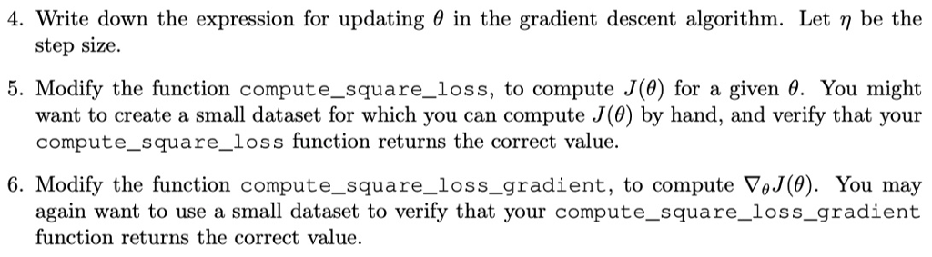
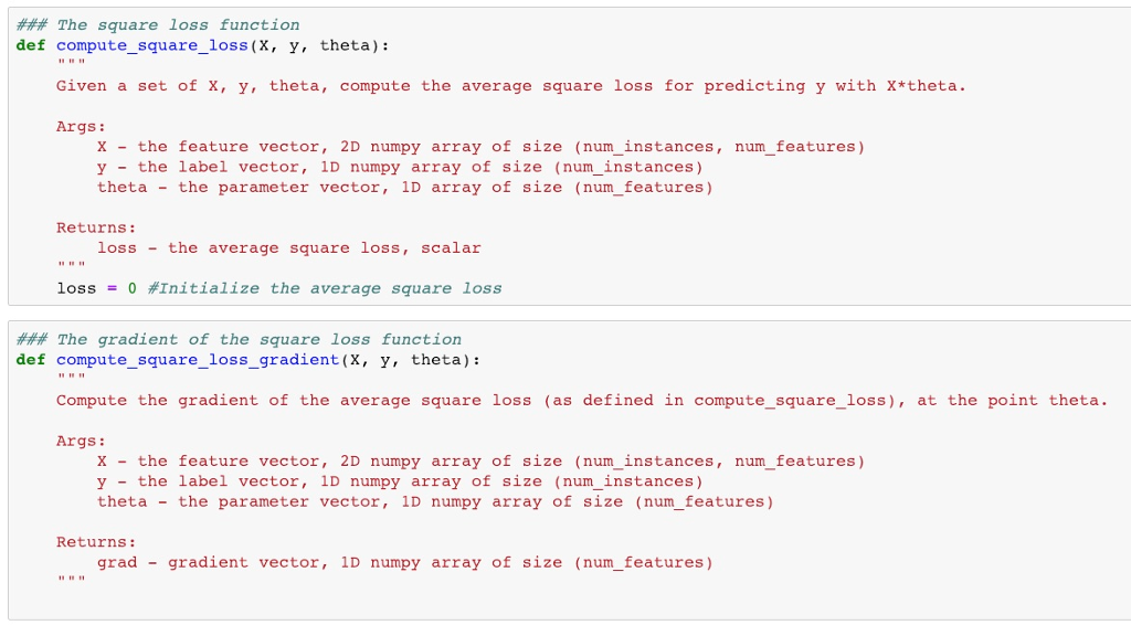
3.2 Gradient Descent Setup In linear regression, we consider the hypothesis space of linear functions ho : Rd - R, where for , x E Rd, and we choose that minimizes the following "average square loss, objective function: where (x1,31), . . . , (Tm,ym) E Rd R is our training data. While this formulation of linear regression is very convenient, it's more standard to use a hy- pothesis space of "affine" functions: which allows a "bias" or nonzero intercept term. The standard way to achieve this, while still maintaining the convenience of the first representation, is to add an extra dimension to x that is always a fixed value, such as 1. You should convince yourself that this is equivalent. We'll assume this representation, and thus we'll actually take x E Rd+1. 1. Let X e Rm*(d+1) be th the ith row of X is z,. Let y e design matrix Where (,.. . , ym) ERmx1 be the "response". Write the objective function J(0) as a matrix/vec- tor expression, without using an explicit summation sign. [Being able to write expressions as matrix/vector expressions without summations is crucial to making implementations that are useful in practice, since you can use numpy (or more generally, an efficient numerical linear algebra library) to implement these matrix/vector operations orders of magnitude faster than naively implementing with loops in Python.] 2. Write down an expression for the gradient of J (again, as a matrix/vector expression, without using an explicit summation sign). 3. In our search for a that minimizes J, suppose we take a step from to + , where h E Rd+1 is the "step direction" (recall, this is not necessarily a unit vector) and E (0,00) is the "step size" (note that this is not the actual length of the step, which is 1hl). Use the gradient to write down an approximate expression for the change in objective function value J( + }) _ J(9). IThis approximation is called a "linear" or "first-order" approximation.] 4. Write down the expression for updating in the gradient descent algorithm. Let be the step size 5. Modify the function compute-square-loss, to compute J(8) for a given . You might want to create a small dataset for which you can compute J(0) by hand, and verify that your compute_square_loss function returns the correct value. 6, Modify the function compute-square-loss-gradient, to compute GJ(). You may again want to use a small dataset to verify that your compute_square_loss_gradient function returns the correct value ### The square loss function def compute_square_loss(X, y, theta): Given a set of x, y, theta, compute the average square loss for predicting y with X*theta. Args: x the feature vector, 2D numpy array of size (num_instances, num_features) y the label vector, 1D numpy array of size (num_instances) theta - the parameter vector,1D array of size (num_ features) Returns: loss - the average square loss, scalar loss = 0 #Initialize the average square loss ### The gradient of the square loss function def compute_square_loss_gradient (x, y, theta): Compute the gradient of the average square loss (as defined in compute_ square_loss), at the point theta. Args: x the feature vector, 2D numpy array of size (num_instances, num_features) y the label vector, 1D numpy array of size (num_instances) theta - the parameter vector, 1D numpy array of size (num features) Returns: grad - gradient vector, 1D numpy array of size (num_features) 3.2 Gradient Descent Setup In linear regression, we consider the hypothesis space of linear functions ho : Rd - R, where for , x E Rd, and we choose that minimizes the following "average square loss, objective function: where (x1,31), . . . , (Tm,ym) E Rd R is our training data. While this formulation of linear regression is very convenient, it's more standard to use a hy- pothesis space of "affine" functions: which allows a "bias" or nonzero intercept term. The standard way to achieve this, while still maintaining the convenience of the first representation, is to add an extra dimension to x that is always a fixed value, such as 1. You should convince yourself that this is equivalent. We'll assume this representation, and thus we'll actually take x E Rd+1. 1. Let X e Rm*(d+1) be th the ith row of X is z,. Let y e design matrix Where (,.. . , ym) ERmx1 be the "response". Write the objective function J(0) as a matrix/vec- tor expression, without using an explicit summation sign. [Being able to write expressions as matrix/vector expressions without summations is crucial to making implementations that are useful in practice, since you can use numpy (or more generally, an efficient numerical linear algebra library) to implement these matrix/vector operations orders of magnitude faster than naively implementing with loops in Python.] 2. Write down an expression for the gradient of J (again, as a matrix/vector expression, without using an explicit summation sign). 3. In our search for a that minimizes J, suppose we take a step from to + , where h E Rd+1 is the "step direction" (recall, this is not necessarily a unit vector) and E (0,00) is the "step size" (note that this is not the actual length of the step, which is 1hl). Use the gradient to write down an approximate expression for the change in objective function value J( + }) _ J(9). IThis approximation is called a "linear" or "first-order" approximation.] 4. Write down the expression for updating in the gradient descent algorithm. Let be the step size 5. Modify the function compute-square-loss, to compute J(8) for a given . You might want to create a small dataset for which you can compute J(0) by hand, and verify that your compute_square_loss function returns the correct value. 6, Modify the function compute-square-loss-gradient, to compute GJ(). You may again want to use a small dataset to verify that your compute_square_loss_gradient function returns the correct value ### The square loss function def compute_square_loss(X, y, theta): Given a set of x, y, theta, compute the average square loss for predicting y with X*theta. Args: x the feature vector, 2D numpy array of size (num_instances, num_features) y the label vector, 1D numpy array of size (num_instances) theta - the parameter vector,1D array of size (num_ features) Returns: loss - the average square loss, scalar loss = 0 #Initialize the average square loss ### The gradient of the square loss function def compute_square_loss_gradient (x, y, theta): Compute the gradient of the average square loss (as defined in compute_ square_loss), at the point theta. Args: x the feature vector, 2D numpy array of size (num_instances, num_features) y the label vector, 1D numpy array of size (num_instances) theta - the parameter vector, 1D numpy array of size (num features) Returns: grad - gradient vector, 1D numpy array of size (num_features)