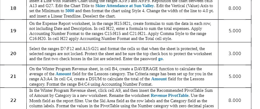
Insert a Line with Markers Chart using the ranges AS:5 and AS.F3. Reposition the Chart between Cells 18 A13 and G27. Edit the Chart Title to Skier Attendance at Sun Valley. Edit the Vertical (Value) Axis to 8.000 set the Minimum to 5000 and then format the chart using Style 4. Change the width of the line to 4.0 pt. and insert a Linear Trendline. Deselect the chart. On the Expense Report worksheet, in the range H15:H21, create formulas to sum the data in each row, 19 not including Date and Description. In cell H22, enter a formula to sum the total expenses. Apply 5.000 Accounting Number Format to the ranges C15:H15 and C21:H21. Apply Comma Style to the range C16:H20. In cell H22 apply Accounting Number Format and the Total cell style. Select the ranges D7:F12 and A15:G21 and format the cells so that when the sheet is protected, the 20 selected ranges are not locked. Protect the sheet and be sure the top check box to protect the worksheet 3.000 and the first two check boxes in the list are selected. Enter the password go. On the Winter Program Revenue sheet, in cell B4, create a DAVERAGE function to calculate the 21 average of the Amount field for the Lessons category. The Criteria range has been set up for you in the 5.000 range A3:A4. In cell C4, create a DSUM to calculate the total of the Amount field for the Lessons category. Format the range B4:C4 using Accounting Number Format. In the Winter Program Revenue sheet, click cell A9, and then insert the Recommended PivotTable Sum of Amount by Category in a new worksheet. Rename the worksheet Revenue PivotTable. Use the 22 Month field as the report filter. Use the Ski Area field as the row labels and the Category field as the 8.000 column labels. Format the values in the PivotTable using the Number category with zero decimal places