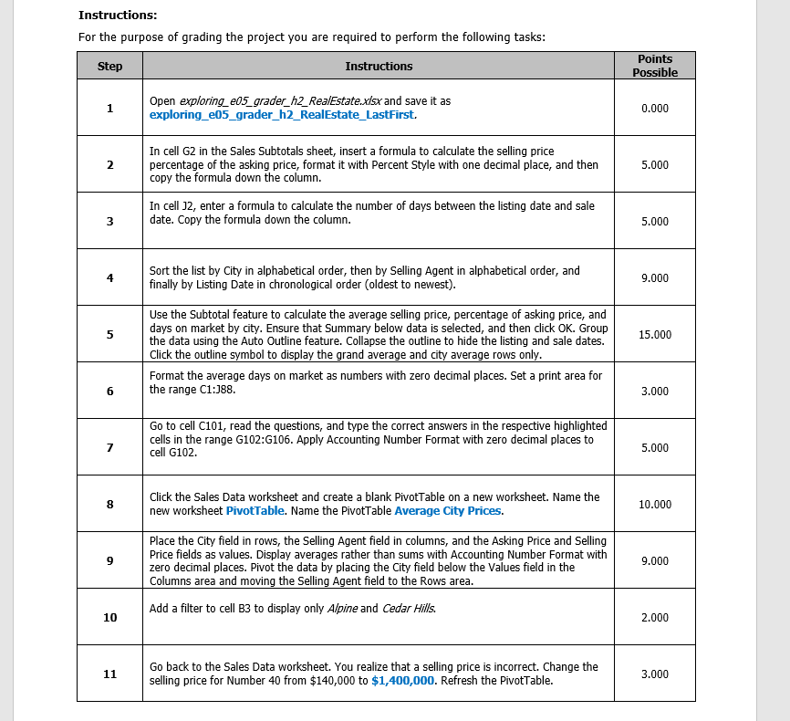
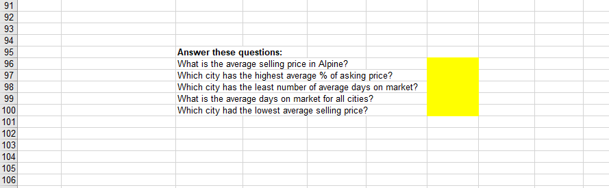
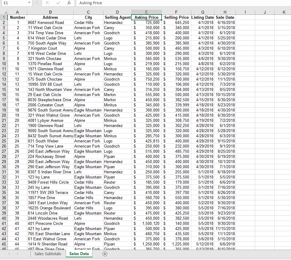
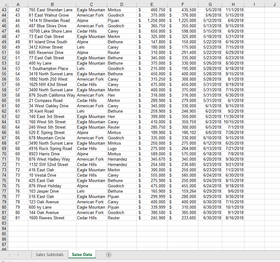
Instructions: For the purpose of grading the project you are required to perform the following tasks: Points Possible Step Open exploring e05_grader h2 RealEstate xis and save it as exploring_e05_grader_h2_RealEstate_LastFirst. 0.000 In cell G2 in the Sales Subtotals sheet, insert a formula to calculate the selling price percentage of the asking price, format it with Percent Style with one decimal place, and then copy the formula down the column. 2 5.000 In cell 12, enter a formula to calculate the number of days between the listing date and sale date. Copy the formula down the column. 3 5.000 Sort the list by City in alphabetical order, then by Selling Agent in alphabetical order, and finally by Listing Date in chronological order (oldest to newest). 4 9.000 Use the Subtotal feature to calculate the average selling price, percentage of asking price, and days on market by city. Ensure that Summary below data is selected, and then click OK. Group the data using the Auto Outline feature. Collapse the outline to hide the listing and sale dates. Click the outline symbol to display the grand average and city average rows onl 5 15.000 Format the average days on market as numbers with zero decimal places. Set a print area for the range C1:188 6 3.000 Go to cell C101, read the questions, and type the correct answers in the respective highlighted cells in the range G102:G106. Apply Accounting Number Format with zero decimal places to cell G102. 5.000 Click the Sales Data worksheet and create a blank PivotTable on a new worksheet. Name the new worksheet PivotTable. Name the PivotTable Average City Prices. 8 10.000 Place the City field in rows, the Selling Agent field in columns, and the Asking Price and Selling Price fields as values. Display averages rather than sums with Accounting Number Format with zero decimal places. Pivot the data by placing the City field below the Values field in the Columns area and moving the Selling Agent field to the Rows area 9 9.000 Add a filter to cell B3 to display only Alpine and Cedar Hills. 10 2.000 Go back to the Sales Data worksheet. You realize that a selling price is incorrect. Change the selling price for Number 40 from $140,000 to $1,400,000. Refresh the PivotTable. 3.000 Instructions: For the purpose of grading the project you are required to perform the following tasks: Points Possible Step Open exploring e05_grader h2 RealEstate xis and save it as exploring_e05_grader_h2_RealEstate_LastFirst. 0.000 In cell G2 in the Sales Subtotals sheet, insert a formula to calculate the selling price percentage of the asking price, format it with Percent Style with one decimal place, and then copy the formula down the column. 2 5.000 In cell 12, enter a formula to calculate the number of days between the listing date and sale date. Copy the formula down the column. 3 5.000 Sort the list by City in alphabetical order, then by Selling Agent in alphabetical order, and finally by Listing Date in chronological order (oldest to newest). 4 9.000 Use the Subtotal feature to calculate the average selling price, percentage of asking price, and days on market by city. Ensure that Summary below data is selected, and then click OK. Group the data using the Auto Outline feature. Collapse the outline to hide the listing and sale dates. Click the outline symbol to display the grand average and city average rows onl 5 15.000 Format the average days on market as numbers with zero decimal places. Set a print area for the range C1:188 6 3.000 Go to cell C101, read the questions, and type the correct answers in the respective highlighted cells in the range G102:G106. Apply Accounting Number Format with zero decimal places to cell G102. 5.000 Click the Sales Data worksheet and create a blank PivotTable on a new worksheet. Name the new worksheet PivotTable. Name the PivotTable Average City Prices. 8 10.000 Place the City field in rows, the Selling Agent field in columns, and the Asking Price and Selling Price fields as values. Display averages rather than sums with Accounting Number Format with zero decimal places. Pivot the data by placing the City field below the Values field in the Columns area and moving the Selling Agent field to the Rows area 9 9.000 Add a filter to cell B3 to display only Alpine and Cedar Hills. 10 2.000 Go back to the Sales Data worksheet. You realize that a selling price is incorrect. Change the selling price for Number 40 from $140,000 to $1,400,000. Refresh the PivotTable. 3.000