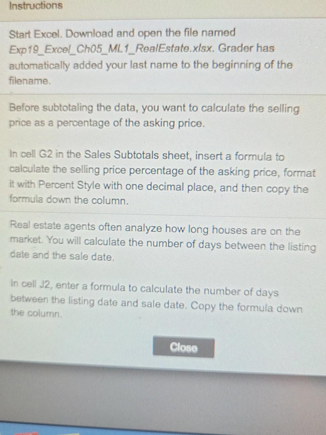
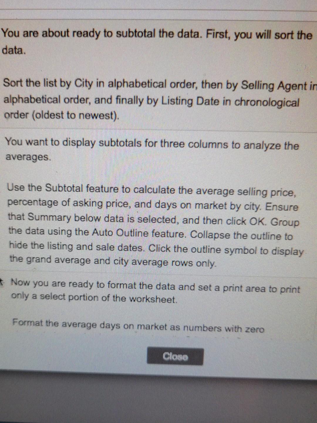
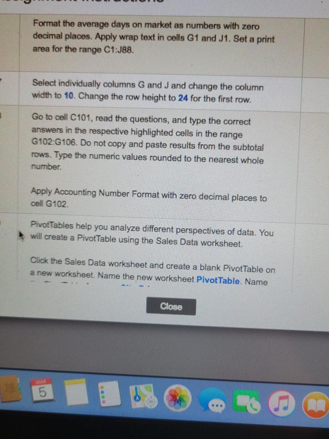
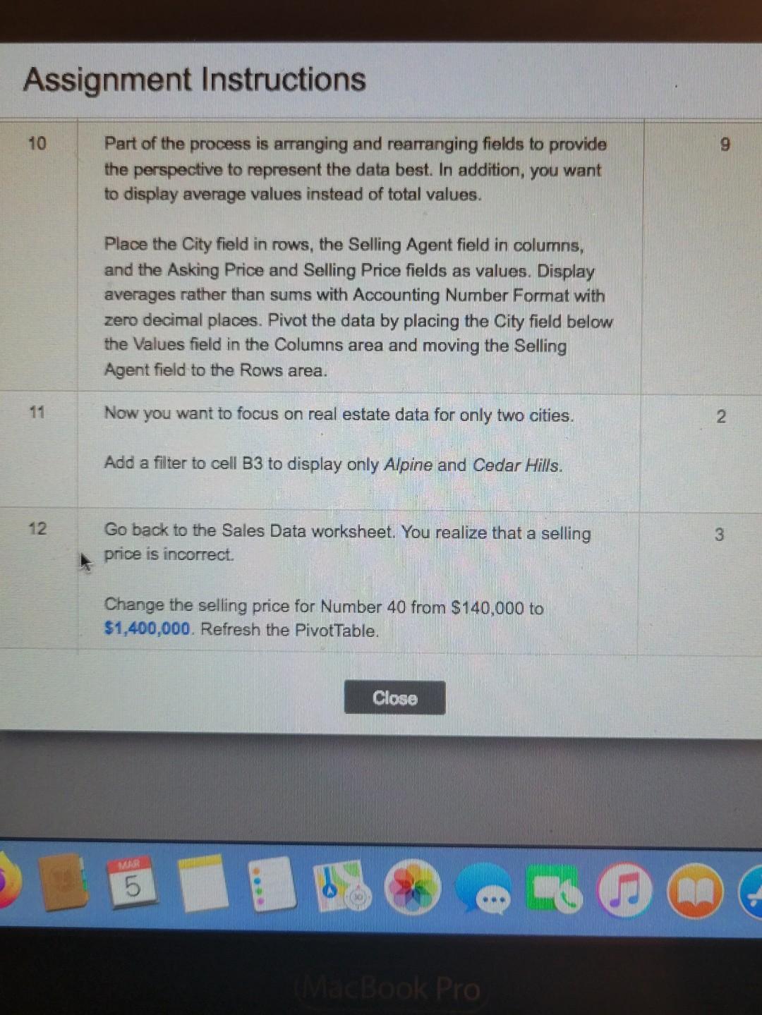
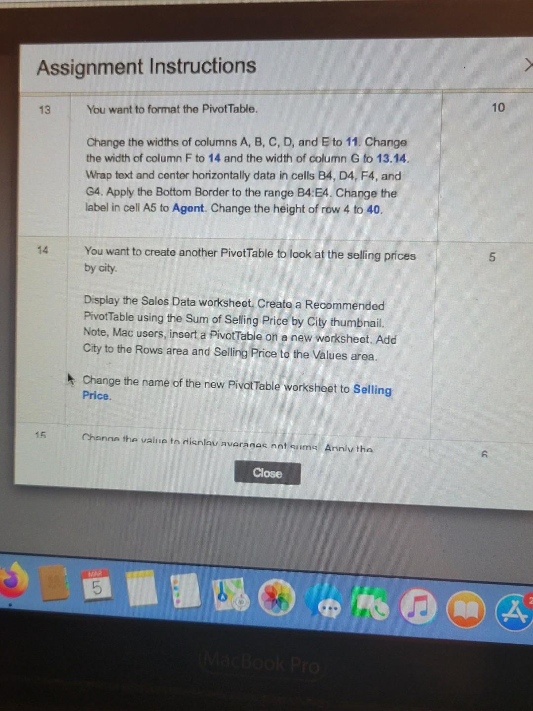
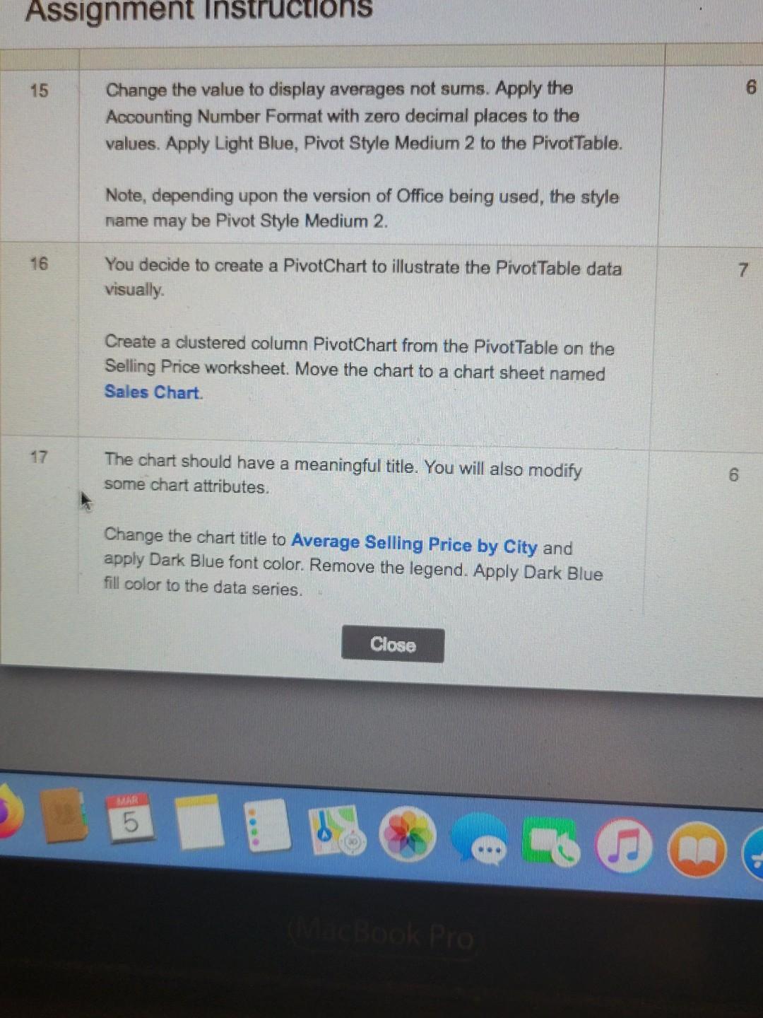
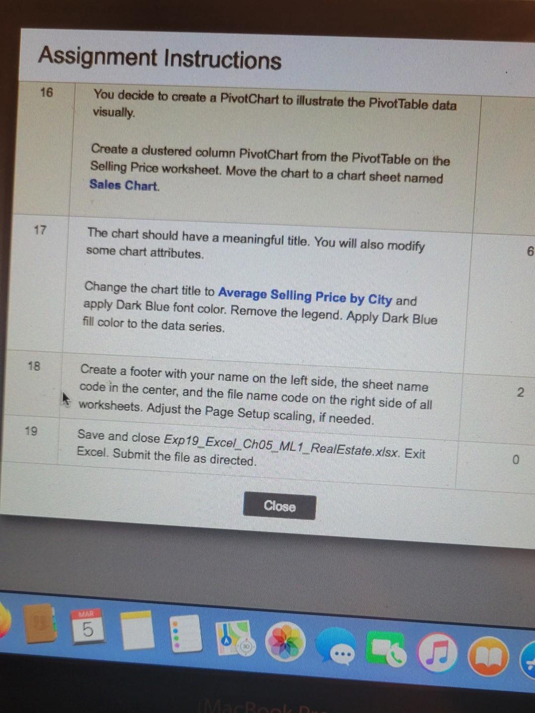
Instructions Start Excel. Download and open the file named Exp19_Excel_Ch05_ML1_RealEstate.xlsx. Grader has automatically added your last name to the beginning of the filename. Before subtotaling the data, you want to calculate the selling price as a percentage of the asking price. In cell G2 in the Sales Subtotals sheet, insert a formula to calculate the selling price percentage of the asking price, format it with Percent Style with one decimal place, and then copy the formula down the column. Real estate agents often analyze how long houses are on the market. You will calculate the number of days between the listing date and the sale date. In cell J2, enter a formula to calculate the number of days between the listing date and sale date. Copy the formula down the column Close You are about ready to subtotal the data. First, you will sort the data. Sort the list by City in alphabetical order, then by Selling Agent in alphabetical order, and finally by Listing Date in chronological order (oldest to newest). You want to display subtotals for three columns to analyze the averages. Use the Subtotal feature to calculate the average selling price, percentage of asking price, and days on market by city. Ensure that Summary below data is selected, and then click OK Group the data using the Auto Outline feature. Collapse the outline to hide the listing and sale dates. Click the outline symbol to display the grand average and city average rows only. Now you are ready to format the data and set a print area to print only a select portion of the worksheet. Format the average days on market as numbers with zero Close Format the average days on market as numbers with zero decimal places. Apply wrap text in cells G1 and J1. Set a print area for the range C1:388. Select individually columns G and J and change the column width to 10. Change the row height to 24 for the first row. Go to cell C101, read the questions, and type the correct answers in the respective highlighted cells in the range G102:G106. Do not copy and paste results from the subtotal rows. Type the numeric values rounded to the nearest whole number. Apply Accounting Number Format with zero decimal places to cell G102. PivotTables help you analyze different perspectives of data. You will create a Pivot Table using the Sales Data worksheet. Click the Sales Data worksheet and create a blank PivotTable on a new worksheet. Name the new worksheet Pivot Table. Name Close MAR 5 Assignment Instructions 10 9 Part of the process is arranging and rearranging fields to provide the perspective to represent the data best. In addition, you want to display average values instead of total values. Place the City field in rows, the Selling Agent field in columns, and the Asking Price and Selling Price fields as values. Display averages rather than sums with Accounting Number Format with zero decimal places. Pivot the data by placing the City field below the Values field in the Columns area and moving the Selling Agent field to the Rows area. Now you want to focus on real estate data for only two cities. 2 Add a filter to cell B3 to display only Alpine and Cedar Hills. 12 Go back to the Sales Data worksheet. You realize that a selling price is incorrect. 3 Change the selling price for Number 40 from $140,000 to $1,400,000. Refresh the Pivot Table, Close 5 MacBook Pro Assignment Instructions 13 You want to format the Pivot Table. 10 Change the widths of columns A, B, C, D, and E to 11. Change the width of column F to 14 and the width of column G to 13.14. Wrap text and center horizontally data in cells B4, D4, F4, and G4. Apply the Bottom Border to the range B4:E4. Change the label in cell A5 to Agent Change the height of row 4 to 40. 14 You want to create another PivotTable to look at the selling prices by city. 5 Display the Sales Data worksheet. Create a Recommended Pivot Table using the Sum of Selling Price by City thumbnail. Note, Mac users, insert a PivotTable on a new worksheet. Add City to the Rows area and Selling Price to the Values area. Change the name of the new Pivot Table worksheet to Selling Price. 15 Channe the value to disnlav averanes not seems Annly the Close MAR X MacBook Pro Assignment Instructions 15 6 Change the value to display averages not sums. Apply the Accounting Number Format with zero decimal places to the values. Apply Light Blue, Pivot Style Medium 2 to the PivotTable. Note, depending upon the version of Office being used, the style name may be Pivot Style Medium 2. 16 7 You decide to create a PivotChart to illustrate the PivotTable data Visually Create a clustered column PivotChart from the Pivot Table on the Selling Price worksheet. Move the chart to a chart sheet named Sales Chart The chart should have a meaningful title. You will also modify some chart attributes. 6 Change the chart title to Average Selling Price by City and apply Dark Blue font color. Remove the legend. Apply Dark Blue fill color to the data series. Close MAR MacBook Pro Assignment Instructions 16 You decide to create a PivotChart to illustrate the Pivot Table data visually Create a clustered column PivotChart from the Pivot Table on the Selling Price worksheet. Move the chart to a chart sheet named Sales Chart 17 The chart should have a meaningful title. You will also modify some chart attributes. 6 Change the chart title to Average Selling Price by City and apply Dark Blue font color. Remove the legend. Apply Dark Blue fill color to the data series. 18 Create a footer with your name on the left side, the sheet name code in the center, and the file name code on the right side of all worksheets. Adjust the Page Setup scaling, if needed. 2. 19 Save and close Exp 19 Excel_Ch05 ML1_RealEstate.xlsx. Exit Excel. Submit the file as directed. 0 Close VER 5 MERolni Instructions Start Excel. Download and open the file named Exp19_Excel_Ch05_ML1_RealEstate.xlsx. Grader has automatically added your last name to the beginning of the filename. Before subtotaling the data, you want to calculate the selling price as a percentage of the asking price. In cell G2 in the Sales Subtotals sheet, insert a formula to calculate the selling price percentage of the asking price, format it with Percent Style with one decimal place, and then copy the formula down the column. Real estate agents often analyze how long houses are on the market. You will calculate the number of days between the listing date and the sale date. In cell J2, enter a formula to calculate the number of days between the listing date and sale date. Copy the formula down the column Close You are about ready to subtotal the data. First, you will sort the data. Sort the list by City in alphabetical order, then by Selling Agent in alphabetical order, and finally by Listing Date in chronological order (oldest to newest). You want to display subtotals for three columns to analyze the averages. Use the Subtotal feature to calculate the average selling price, percentage of asking price, and days on market by city. Ensure that Summary below data is selected, and then click OK Group the data using the Auto Outline feature. Collapse the outline to hide the listing and sale dates. Click the outline symbol to display the grand average and city average rows only. Now you are ready to format the data and set a print area to print only a select portion of the worksheet. Format the average days on market as numbers with zero Close Format the average days on market as numbers with zero decimal places. Apply wrap text in cells G1 and J1. Set a print area for the range C1:388. Select individually columns G and J and change the column width to 10. Change the row height to 24 for the first row. Go to cell C101, read the questions, and type the correct answers in the respective highlighted cells in the range G102:G106. Do not copy and paste results from the subtotal rows. Type the numeric values rounded to the nearest whole number. Apply Accounting Number Format with zero decimal places to cell G102. PivotTables help you analyze different perspectives of data. You will create a Pivot Table using the Sales Data worksheet. Click the Sales Data worksheet and create a blank PivotTable on a new worksheet. Name the new worksheet Pivot Table. Name Close MAR 5 Assignment Instructions 10 9 Part of the process is arranging and rearranging fields to provide the perspective to represent the data best. In addition, you want to display average values instead of total values. Place the City field in rows, the Selling Agent field in columns, and the Asking Price and Selling Price fields as values. Display averages rather than sums with Accounting Number Format with zero decimal places. Pivot the data by placing the City field below the Values field in the Columns area and moving the Selling Agent field to the Rows area. Now you want to focus on real estate data for only two cities. 2 Add a filter to cell B3 to display only Alpine and Cedar Hills. 12 Go back to the Sales Data worksheet. You realize that a selling price is incorrect. 3 Change the selling price for Number 40 from $140,000 to $1,400,000. Refresh the Pivot Table, Close 5 MacBook Pro Assignment Instructions 13 You want to format the Pivot Table. 10 Change the widths of columns A, B, C, D, and E to 11. Change the width of column F to 14 and the width of column G to 13.14. Wrap text and center horizontally data in cells B4, D4, F4, and G4. Apply the Bottom Border to the range B4:E4. Change the label in cell A5 to Agent Change the height of row 4 to 40. 14 You want to create another PivotTable to look at the selling prices by city. 5 Display the Sales Data worksheet. Create a Recommended Pivot Table using the Sum of Selling Price by City thumbnail. Note, Mac users, insert a PivotTable on a new worksheet. Add City to the Rows area and Selling Price to the Values area. Change the name of the new Pivot Table worksheet to Selling Price. 15 Channe the value to disnlav averanes not seems Annly the Close MAR X MacBook Pro Assignment Instructions 15 6 Change the value to display averages not sums. Apply the Accounting Number Format with zero decimal places to the values. Apply Light Blue, Pivot Style Medium 2 to the PivotTable. Note, depending upon the version of Office being used, the style name may be Pivot Style Medium 2. 16 7 You decide to create a PivotChart to illustrate the PivotTable data Visually Create a clustered column PivotChart from the Pivot Table on the Selling Price worksheet. Move the chart to a chart sheet named Sales Chart The chart should have a meaningful title. You will also modify some chart attributes. 6 Change the chart title to Average Selling Price by City and apply Dark Blue font color. Remove the legend. Apply Dark Blue fill color to the data series. Close MAR MacBook Pro Assignment Instructions 16 You decide to create a PivotChart to illustrate the Pivot Table data visually Create a clustered column PivotChart from the Pivot Table on the Selling Price worksheet. Move the chart to a chart sheet named Sales Chart 17 The chart should have a meaningful title. You will also modify some chart attributes. 6 Change the chart title to Average Selling Price by City and apply Dark Blue font color. Remove the legend. Apply Dark Blue fill color to the data series. 18 Create a footer with your name on the left side, the sheet name code in the center, and the file name code on the right side of all worksheets. Adjust the Page Setup scaling, if needed. 2. 19 Save and close Exp 19 Excel_Ch05 ML1_RealEstate.xlsx. Exit Excel. Submit the file as directed. 0 Close VER 5 MERolni