INSTRUCTIONS There are three parts to this project in Python. Please read all sections of the instructions carefully.

I. Perceptron Learning Algorithm II. Linear Regression III. Classification

You are allowed to use Python packages to help you solve the problems and plot any results for reference, including numpy, scipy, pandas and scikit-learn. For optional problems, you may find matplotlib package useful. However, please do NOT submit any code using Tkinter, matplotlib, seaborn, or any other plotting library.

I. Perceptron Learning Algorithm In this question, you will implement the Perceptron Learning Algorithm ("PLA") for a linearly separable dataset. In your starter code, you will find input1.csv, containing a series of data points. Each point is a comma-separated ordered triple, representing feature_1, feature_2, and the label for the point. You can think of the values of the features as the x- and y-coordinates of each point. The label takes on a value of positive or negative one. You can think of the label as separating the points into two categories. Implement your PLA in a file called problem1.py, which will be executed like so:

$ python problem1.py input1.csv output1.csv

If you are using Python3, name your file problem1_3.py, which will be executed like so:

$ python3 problem1_3.py input1.csv output1.csv

This should generate an output file called output1.csv. With each iteration of your PLA (each time we go through all examples), your program must print a new line to the output file, containing a comma-separated list of the weights w_1, w_2, and b in that order. Upon convergence, your program will stop, and the final values of w_1, w_2, and b will be printed to the output file (for an example see output1.csv). This defines the decision boundary that your PLA has computed for the given dataset.

Note: When implementing your PLA, in case of tie (sum of w_jx_ij = 0), please follow the lecture note and classify the datapoint as -1.

What To Submit. problem1.py or problem1_3.py, which should behave as specified above.

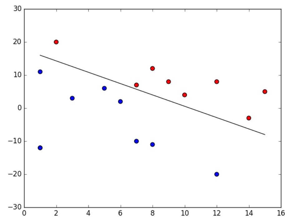
Optional (0 pts). To visualize the progress and final result of your program, you can use matplotlib to output an image for each iteration of your algorithm. For instance, you can plot each category with a different color, and plot the decision boundary with its equation. An example is shown above for reference.

II. Linear Regression In this problem, you will work on linear regression with multiple features using gradient descent. In your starter code, you will find input2.csv, containing a series of data points. Each point is a comma-separated ordered triple, representing age, weight, and height (derived from CDC growth charts data).

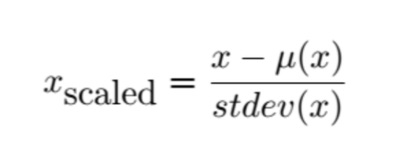
Data Preparation and Normalization. Once you load your dataset, explore the content to identify each feature. Remember to add the vector 1 (intercept) ahead of your data matrix. You will notice that the features are not on the same scale. They represent age (years), and weight (kilograms). What is the mean and standard deviation of each feature? The last column is the label, and represents the height (meters). Scale each feature (i.e. age and weight) by its (population) standard deviation, and set its mean to zero. (Can you see why this will help?) You do not need to scale the intercept.

For each feature x (a column in your data matrix), use the following formula for scaling:

Gradient Descent. Implement gradient descent to find a regression model. Initialize your s to zero. Recall the empirical risk and gradient descent rule as follows:

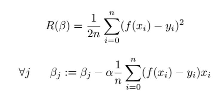
Run the gradient descent algorithm using the following learning rates: {0.001, 0.005, 0.01, 0.05, 0.1, 0.5, 1, 5, 10}. For each value of , run the algorithm for exactly 100 iterations. Compare the convergence rate when is small versus large. What is the ideal learning rate to obtain an accurate model? In addition to the nine learning rates above, come up with your own choice of value for the learning rate. Then, using this new learning rate, run the algorithm for your own choice of number of iterations.

Implement your gradient descent in a file called problem2.py, which will be executed like so:

$ python problem2.py input2.csv output2.csv

If you are using Python3, name your file problem2_3.py, which will be executed like so:

$ python3 problem2_3.py input2.csv output2.csv

This should generate an output file called output2.csv. There are ten cases in total, nine with the specified learning rates (and 100 iterations), and one with your own choice of learning rate (and your choice of number of iterations). After each of these ten runs, your program must print a new line to the output file, containing a comma-separated list of alpha, number_of_iterations, b_0, b_age, and b_weight in that order (for an example see output2.csv), expressed with as many decimal places as you please. These represent the regression models that your gradient descents have computed for the given dataset.

What To Submit. problem2.py or problem2_3.py, which should behave as specified above.

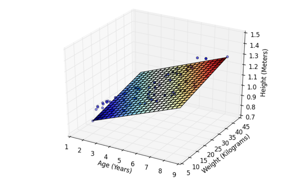
Optional (0 pts). To visualize the result of each case of gradient descent, you can use matplotlib to output an image for each linear regression model in three-dimensional space. For instance, you can plot each feature on the xy-plane, and plot the regression equation as a plane in xyz-space. An example is shown above for reference.

III. Classification In this problem you will use the support vector classifiers in the sklearn package to learn a classification model for a chessboard-like dataset. In your starter code, you will find input3.csv, containing a series of data points. Open the dataset in python. Make a scatter plot of the dataset showing the two classes with two different patterns.

Use SVM with different kernels to build a classifier. Make sure you split your data into training (60%) and testing (40%). Also make sure you use stratified sampling (i.e. same ratio of positive to negative in both the training and testing datasets). Use cross validation (with the number of folds k = 5) instead of a validation set. You do not need to scaleormalize the data for this question. Train-test splitting and cross validation functionalities are all readily available in sklearn.

SVM with Linear Kernel. Observe the performance of the SVM with linear kernel. Search for a good setting of parameters to obtain high classification accuracy. Specifically, try values of C = [0.1, 0.5, 1, 5, 10, 50, 100]. Read about sklearn.grid_search and how this can help you accomplish this task. After locating the optimal parameter value by using the training data, record the corresponding best score (training data accuracy) achieved. Then apply the testing data to the model, and record the actual test score. Both scores will be a number between zero and one.

SVM with Polynomial Kernel. (Similar to above). Try values of C = [0.1, 1, 3], degree = [4, 5, 6], and gamma = [0.1, 0.5].

SVM with RBF Kernel. (Similar to above). Try values of C = [0.1, 0.5, 1, 5, 10, 50, 100] and gamma = [0.1, 0.5, 1, 3, 6, 10].

Logistic Regression. (Similar to above). Try values of C = [0.1, 0.5, 1, 5, 10, 50, 100].

k-Nearest Neighbors. (Similar to above). Try values of n_neighbors = [1, 2, 3, ..., 50] and leaf_size = [5, 10, 15, ..., 60].

Decision Trees. (Similar to above). Try values of max_depth = [1, 2, 3, ..., 50] and min_samples_split = [2, 3, 4, ..., 10].

Random Forest. (Similar to above). Try values of max_depth = [1, 2, 3, ..., 50] and min_samples_split = [2, 3, 4, ..., 10].

What To Submit. problem2.py or problem2_3.py along with output3.csv (for an example see output3.csv). The output3.csv file should contain an entry for each of the seven methods used. For each method, print a comma-separated list as shown in the example, including the method name, best score, and test score, expressed with as many decimal places as you please. There may be more than one way to implement a certain method, and we will allow for small variations in output you may encounter depending on the specific functions you decide to use.

input1.csv

8	-11	1
7	7	-1
12	-20	1
14	-3	-1
12	8	-1
1	-12	1
15	5	-1
7	-10	1
10	4	-1
6	2	1
8	12	-1
2	20	-1
1	-12	1
9	8	-1
3	3	1
5	6	1
1	11	1

input2.csv

2	10.21027	0.8052476
2.04	13.07613	0.9194741
2.13	11.44697	0.9083505
2.21	14.43984	0.8037555
2.29	12.59622	0.811357
2.38	10.5199	0.9489974
2.46	12.89517	0.9664505
2.54	12.11692	0.9288403
2.63	16.76085	0.86205
2.71	11.20934	0.9811632
2.79	13.48913	0.9883778
2.88	11.85574	1.004748
2.96	11.54332	1.001915
3.04	12.90222	0.9934899
3.13	13.03542	0.8974875
3.21	11.88202	0.8887256
3.29	11.99685	0.932307
3.38	11.82981	0.937784
3.46	12.70158	1.05032
3.54	19.58748	1.056727
3.63	16.46093	0.9821247
3.71	15.20721	0.91031
3.79	15.37263	1.065316
3.88	14.29485	1.02835
3.96	13.47689	0.9255748
4.04	13.61116	0.9306862
4.13	13.21864	1.101614
4.21	13.02441	0.9921132
4.29	18.04961	1.114548
4.38	18.25533	1.063936
4.46	13.40907	1.008634
4.54	15.51193	1.044635
4.63	15.66975	1.140624
4.71	17.28859	0.9824303
4.79	14.29081	1.062029
4.88	21.63373	1.100134
4.96	14.20687	1.166945
5.04	14.34277	1.161301
5.13	20.16834	1.009289
5.21	25.58315	1.091316
5.29	18.58571	1.097202
5.38	14.8925	1.025529
5.46	16.06749	1.076194
5.54	15.56413	1.114876
5.63	25.83467	1.187193
5.71	17.81035	1.09323
5.79	15.58975	1.069648
5.88	16.83304	1.173466
5.96	15.87089	1.232684
6.04	16.43608	1.057615
6.13	22.90029	1.245461
6.21	28.0358	1.251804
6.29	29.97981	1.167406
6.38	26.52102	1.089877
6.46	21.35797	1.215447
6.54	17.3225	1.118232
6.63	29.70296	1.123483
6.71	30.04782	1.110545
6.79	20.11027	1.309295
6.88	18.73445	1.108909
6.96	22.64564	1.175754
7.04	18.22805	1.149112
7.13	18.38153	1.135427
7.21	32.20984	1.339077
7.29	18.16912	1.330256
7.38	19.73432	1.313696
7.46	19.00511	1.173512
7.54	27.35114	1.159026
7.63	22.04564	1.367356
7.71	19.48502	1.168069
7.79	19.64775	1.263869
7.88	19.23024	1.368565
7.96	20.96755	1.388876
8.04	33.19435	1.318567
8.13	20.31464	1.384097
8.21	29.81185	1.213855
8.29	20.65887	1.218047
8.38	26.82559	1.414521
8.46	40.94614	1.301148

A	B	label
3.4	0.35	1
0.7	0.2	1
3.55	2.5	0
3.1	0.35	1
0.7	1.3	1
3.2	1.4	0
2.15	1.85	1
0.2	2.4	0
1.9	3.15	0
0.25	2.5	0
2.5	0.65	0
0.8	1.15	1
1.15	1.65	0
3.15	1.85	0
3.45	1.2	1
1.9	1.25	0
2.3	3.55	0
3.15	1.2	1
0.9	2.25	0
0.85	3.5	1
2.6	1.8	1
3.15	3.7	1
2.5	1.45	1
1.15	3.4	1
0.3	3.8	1
1.3	1.1	1
0	3.85	1
1.45	0.6	0
0	0.15	1
2.3	2.55	1
0.25	3.05	1
3.4	2.1	0
4	1.5	0
1.9	0.45	0
3.8	1.85	0
3.95	0.4	1
2.85	0.55	1
3.85	2	0
1.15	0.9	1
2.8	3.5	1
2.8	2.65	0
2.2	3	0
3.25	3.05	1
0.45	1.6	0
2.1	0.9	0
0.7	2.6	0
0.85	2.55	0
2.7	1.15	1
2.85	0.3	1
3.55	1.05	1
3.35	3.9	1
2.95	3.05	1
3.7	2.95	1
3.3	0.25	1
2.2	2.65	1
3.35	2.15	0
1.8	2.75	0
2	2.6	1
2.55	3.1	0
0.4	3.35	1
3.65	1.8	0
3.95	2.2	0
3	1	1
0	2.85	1
1.1	0.85	1
3.4	1.75	0
1.5	0.25	0
1.4	3.1	0
1.35	1.9	1
0.2	3.6	1
2.7	3.2	1
2.05	0.45	0
2.35	1.35	1
1.9	0.6	0
1.05	2.4	0
1.55	2.9	0
3.55	0	1
2.55	0.35	0
0.3	2.55	0
3.95	3.5	1
3.65	0.15	1
3.7	1.15	1
2.4	3.45	0
1.4	2.7	0
1.55	3.65	0
1.15	3.75	1
2.1	3.35	0
3.9	3.3	1
3.35	1.7	0
3.5	3.25	1
2.45	2.05	1
1.9	2.5	1
1.1	3.15	1
3.45	3.05	1
3.6	3.3	1
3	3.95	1
2.2	1.85	1
1.35	1.4	1
2	2.35	1
0.4	2.9	1
3.05	2.2	0
3.2	1.7	0
2.8	0.05	1
3.05	3.35	1
1.5	2.45	1
0.25	2.65	0
1	1.25	1
0.8	3.05	1
3.7	1.85	0
1.65	2.85	0
1.85	3.4	0
3.75	3.7	1
1.45	0.9	0
2.15	3	0
1.5	1.35	1
0.95	3.85	1
1	0.9	1
1.3	0.25	1
1.7	3.65	0
1.7	2.4	1
3.9	2	0
2.85	0.25	1
3.8	3.85	1
3.15	2.7	1
2.8	1.65	0
1.1	0.15	1
3.65	2	0
2.9	1.05	1
3	0.15	1
0.9	1.25	1
0.45	0.7	1
1.55	3.55	0
2.8	4	1
2.45	2	1
1.95	1.6	1
0.6	3.15	1
2.55	3.45	0
2.8	1	1
3.95	0	1
0.45	1.85	0
3.35	0.8	1
0.4	0.3	1
2.1	2.05	1
3.95	3.15	1
2.4	1.1	0
3.35	0.15	1
0.05	0.5	1
1.9	0.2	0
3.6	3	1
3.8	1.2	1
1.8	3.2	0
1.35	1.55	1
3.6	2.7	1
0.85	3.6	1
3.85	2.1	0
3	2.5	0
0.75	2.4	0
2.15	0.3	0
1.1	1.35	0
4	3.15	1
3.15	1.25	1
2.6	2.4	1
1.75	1.1	0
0.6	2.25	0
3.3	3.65	1
0.65	1.15	1
2.5	0.6	0
3.2	0.55	1
2.8	3.65	1
0.85	3.7	1
1.2	1.85	0
3.45	3.5	1
0.5	1.4	0
3.2	0.6	1
1.45	2.5	1
1	2.85	1
3.6	1.1	1
0.85	1.15	1
1.85	3.35	0
2.25	3	0
3.55	3.6	1
1	2.9	1
1.05	0.15	1
1.3	3.3	1
2.7	3.5	1
0.6	2.3	0
0.15	2	0
3.2	0.5	1
0	2.95	1
2.2	3.05	0
2.15	3.3	0
3.05	2.6	0
1.3	3.7	1
3.05	3.65	1
1.8	3.6	0
2.65	3.6	0
3.05	1.6	0
1.7	0.8	0
0.4	3.25	1
2.35	2.6	1
2.1	0.7	0
3.65	2.55	0
2.6	1.25	0
1.5	0.8	0
1.5	2.4	1
1.85	3.6	0
3.4	1.5	0
1.05	1.2	1
0.7	0.4	1
0.2	2.85	1
0.15	0	1
2.75	3.85	1
2.25	1.5	1
1.9	1.45	1
0.2	0.15	1
2.35	3.5	0
0.15	3.05	1
2.65	3.55	0
2.25	3.25	0
2.85	0.2	1
3.8	0.8	1
2.7	1.75	0
1.95	3.15	0
2.7	1.1	1
0.1	1.05	1
1.45	2.65	1
2.7	2.6	0
0.75	1.4	0
3	1.05	1
0.15	3.15	1
0.8	3.8	1
2	3.45	0
3.35	1	1
0.2	2.9	1
1.6	1.55	1
2.45	1.8	1
0.35	2	0
0.5	2.65	0
1.45	1.95	1
2	3	0
1.15	2.1	0
2.3	0.85	0
0.6	0.3	1
2.95	3.6	1
0.8	3	1
3.4	0.65	1
2.35	0.85	0
1.1	0.6	1
2.65	2.55	1
3.6	0.5	1
0.6	1.85	0
0.2	0.55	1
1.75	1.2	0
1.25	1.3	1
2.2	3.25	0
3.7	2.75	1
0.9	1.3	1
1.8	1	0
1.55	1.7	1
0.6	1.35	0
1.3	0.75	1
3.6	1.95	0
2.35	1.3	0
0.7	2.3	0
3.85	3.7	1
3	2	0
0.85	3.1	1
3.4	3.55	1
2.1	3	0
3.9	3.9	1
1.5	1	0
2.2	1.9	1
0.25	0.55	1
3.8	2.15	0
2.65	3.15	0
3.1	0.65	1
1.6	1.15	0
1.55	1.8	1
3.9	0	1
2.15	3.6	0
2.25	2.15	1
1.5	1.55	1
3.15	2.5	0
2	3.75	0
1.65	2.55	1
0.05	3.8	1
4	1.25	1
4	0.7	1
1.15	3.5	1
3.65	3.6	1
3.1	0.9	1
3.95	0.9	1
0.95	1.65	0
2.3	0.95	0
0.85	3.2	1
2.25	1.15	0
2.1	2.15	1
0.85	1.7	0
1.9	3.9	0
0.25	1.75	0
1.35	2.45	1
3.2	0.9	1
0.3	1.1	1
3.8	4	1
0.35	1.85	0
2.95	0.9	1
3.05	2	0
0.85	1.35	0
0.75	3	1
0.2	3.2	1
1.6	2.4	1
1.1	0.05	1
1.1	3.35	1
0.45	2.95	1
0.95	2.85	1
3.85	3.6	1
3.85	3.45	1
3.85	3.75	1
0.4	1.8	0
3.65	2.65	0
1.8	3.55	0
3.75	0.3	1
0	1.75	0
3.7	3.2	1
2.3	0.7	0
1.55	3.85	0
3.9	1.05	1
1.55	2.75	0
3	1.1	1
1.15	3.9	1
0.6	3.65	1
1.15	1.1	1
2.2	0.85	0
0.15	2.65	0
2.4	3.2	0
0.05	3.4	1
3.2	1.1	1
2.45	0.4	0
2.95	3.95	1
3.6	0.3	1
0.65	0.7	1
0.95	0.7	1
1.5	1.25	0
2.35	0.5	0
0.05	3.35	1
2.35	0.9	0
0.65	0.8	1
3.95	3.9	1
0.2	3.4	1
2.55	1.65	1
2	0.5	0
1.15	3.65	1
2	1.8	1
2.8	0.4	1
1.2	3.65	1
2.45	2.5	1
1.95	3.65	0
1.1	0.9	1
0.2	0.25	1
3.7	3.9	1
3.35	2.85	1
3.35	0.25	1
2.55	0.25	0
0.4	2.3	0
1.45	2.85	0
0.55	1.95	0
0.55	0.45	1
1.55	0.65	0
3.9	0.3	1
0.75	1.05	1
1.15	1.3	1
0.35	2.6	0
2.25	3.8	0
1.05	1.5	0
1.6	0.4	0
2.05	1.3	0
3.3	3.85	1
3.75	4	1
3.6	2.45	0
2.25	0.95	0
0.5	1.15	1
0.15	0.3	1
1	3.4	1
2.8	1.25	1
2.95	1.75	0
3.2	3.2	1
2.05	2.45	1
2.5	2.95	0
2.15	2.95	0
4	1.85	0
0.6	2.4	0
1.95	1.1	0
0.95	0.95	1
2	2.25	1
0.05	1.9	0
1.25	2.85	1
3.15	2.35	0
3.4	1.05	1
2.5	1	0
3.25	2.35	0
1.55	0.7	0
3.95	1.35	0
1.65	0.15	0
3.75	0.35	1
2.15	3.25	0
2.75	4	1
1.8	2.95	0
1.5	1.3	0
1.25	1.85	0
0	1.9	0
3.8	1	1
1.55	1.4	1
3.8	3.7	1
2.85	1.15	1
1.4	1.85	1
1	0.65	1
2.6	1.5	1
4	3.25	1
0.25	2.3	0
3.05	3	1
1.65	0.95	0
0.75	0.85	1
2.6	0.2	0
1.7	3.15	0
1.6	2.3	1
3.45	3.3	1
0.35	0.45	1
2.9	0.4	1
0.3	3	1
1.75	1.75	1
2.1	2.8	0
3.1	3.4	1
2.65	0.5	0
1.05	3.25	1
3.95	1.45	0
1	0.05	1
0.95	3.45	1
1.35	1.85	1
3.2	1	1
2.3	3.25	0
1.85	3.1	0
3.45	3.35	1
3.55	3	1
1.45	2.9	0
3.6	3.7	1
1	1.7	0
3.7	1.25	1
2.35	3.35	0
0.85	3.15	1
0.4	2.15	0
1.05	0.75	1
0.75	1.2	1
0.6	1.05	1
0.05	1.2	1
2.15	0.9	0
0.15	1	1
0.65	0.65	1
0.8	2.95	1
2.55	2.6	1
4	0.8	1
2.2	1.75	1
0.85	1.8	0
3.9	0.95	1
4	1.35	0
0.8	1.3	1
0.8	0.1	1
1.85	1.95	1
1.4	1.5	1
3.3	1.65	0
1.45	2.75	0
3.25	2.05	0
2.7	0.75	1
2.15	3.5	0
0.35	1.65	0
3.55	1.45	0
1.75	1.65	1
1	2.3	0
3.65	0.1	1
2.75	2.05	0
1.05	0.3	1
0.15	4	1
0.95	0.8	1
0.2	0.65	1
3.25	1.25	1
2.15	2.3	1
3.65	0.9	1
3.85	0.35	1
1.5	0.7	0
2.35	3	0
0.55	3.85	1
0.95	1.15	1
0.95	0.5	1
1.55	2.6	1
1.4	0.55	0
1.85	1.05	0
2.75	1.8	0
2	0.4	0
2.35	2.7	0
0.95	2.65	0
3.95	0.2	1

0.001	100	[b_0]	[b_age]	[b_weight]
0.005	100	[b_0]	[b_age]	[b_weight]
0.01	100	[b_0]	[b_age]	[b_weight]
0.05	100	[b_0]	[b_age]	[b_weight]
0.1	100	[b_0]	[b_age]	[b_weight]
0.5	100	[b_0]	[b_age]	[b_weight]
1	100	[b_0]	[b_age]	[b_weight]
5	100	[b_0]	[b_age]	[b_weight]
10	100	[b_0]	[b_age]	[b_weight]
[your_choice]	[your_choice]	[b_0]	[b_age]	[b_weight]

30 20 10 -10 20 30 10 12 14 16