intructions are provided

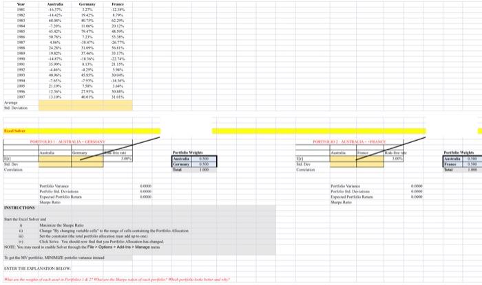
The Excel supplement has the returns of three market indices - Australia, Germany, and France from 1981 to 1997. Please provide the Excel file with your submission. Question: Obtain the mean (expected) and standard deviations of all market indices using "=Average" and "=Std.S" in the yellow cells (B19:D20). You will create two optimal risky portfolios. Portfolio 1 has Australia and Germany. Portfolio 2 has Australia and France. To create these portfolios you need to enter the inputs in the relevant places and then use the Excel Solver to find the optimal portfolio. Below is the guideline to create Portfolio 1 (Australia + Germany) : B29 and B30 should be the expected (mean) return and standard deviation of the Australian market index respectively. C29 and C30 should be the expected (mean) return and standard deviation of the German market index respectively. B31 is the correlation between Australia and Germany. To compute the correlation, use "=CORREL(B2:B18, C2:C18)", which gives the correlation between the Australian and German indices stock returns from 1981 to 1997. Cells E34 to E37 give the variance, expected return, and Sharpe ratio of portfolio 1. Note that weights in H29 and H30 are initially arbitrary ( 50% in Australia. 50% in Germany). Now the task is to create our optimal portfolio (i.e. the one with the highest possible Sharpe ratio.) Open the Solver dialogue box from the tools menu. If the Solver option is not found in the tools menu, Solve will need to be added to the Excel software. Refer to the Help menu in Excel for how to add the Solver function. Our goal is to maximize the value of the Sharpe ratio (cell E37) by changing the weights of the assets in the portfolio (cells H29:H30). So, in the dialogue box, chose cell E37 in the "Set objective" area, and chose the MAX option. In the "By changing variable cells" area, chose H29:H30. When you press Solve, asset weights will change and show the ones in the optimal risky portfolio. Implement the same procedure for Portfolio 2. What are the weights of each asset in Portfolios 1 \& 2? What are the Sharpe ratios of each portfolio? Which portfolio looks better and why? (Please enter the explanation/answer in the Excel file) The Excel supplement has the returns of three market indices - Australia, Germany, and France from 1981 to 1997. Please provide the Excel file with your submission. Question: Obtain the mean (expected) and standard deviations of all market indices using "=Average" and "=Std.S" in the yellow cells (B19:D20). You will create two optimal risky portfolios. Portfolio 1 has Australia and Germany. Portfolio 2 has Australia and France. To create these portfolios you need to enter the inputs in the relevant places and then use the Excel Solver to find the optimal portfolio. Below is the guideline to create Portfolio 1 (Australia + Germany) : B29 and B30 should be the expected (mean) return and standard deviation of the Australian market index respectively. C29 and C30 should be the expected (mean) return and standard deviation of the German market index respectively. B31 is the correlation between Australia and Germany. To compute the correlation, use "=CORREL(B2:B18, C2:C18)", which gives the correlation between the Australian and German indices stock returns from 1981 to 1997. Cells E34 to E37 give the variance, expected return, and Sharpe ratio of portfolio 1. Note that weights in H29 and H30 are initially arbitrary ( 50% in Australia. 50% in Germany). Now the task is to create our optimal portfolio (i.e. the one with the highest possible Sharpe ratio.) Open the Solver dialogue box from the tools menu. If the Solver option is not found in the tools menu, Solve will need to be added to the Excel software. Refer to the Help menu in Excel for how to add the Solver function. Our goal is to maximize the value of the Sharpe ratio (cell E37) by changing the weights of the assets in the portfolio (cells H29:H30). So, in the dialogue box, chose cell E37 in the "Set objective" area, and chose the MAX option. In the "By changing variable cells" area, chose H29:H30. When you press Solve, asset weights will change and show the ones in the optimal risky portfolio. Implement the same procedure for Portfolio 2. What are the weights of each asset in Portfolios 1 \& 2? What are the Sharpe ratios of each portfolio? Which portfolio looks better and why? (Please enter the explanation/answer in the Excel file)