

Question
ISyE 7406: Data Mining & Statistical Learning HW#4 Local Smoothing in R. The goal of this homework is to help you better understand the statistical
ISyE 7406: Data Mining & Statistical Learning HW#4 Local Smoothing in R. The goal of this homework is to help you better understand the statistical properties and computational challenges of local smoothing such as loess, Nadaraya-Watson (NW) kernel smoothing, and spline smoothing. For this purpose, we will compute empirical bias and empirical variances based on m = 1000 Monte Carlo runs, where in each run we simulate a data set of n = 101 observations from the additive model Yi = f(xi) + i (1) with the famous Mexican hat function f(x) = (1 x 2 ) exp(0.5x 2 ), 2 x 2, (2) and 1, , n are independent and identically distributed (iid) N(0, 0.2 2 ). This function is known to pose a variety of estimation challenges, and below we explore the difficulties inherent in this function. (1) Let us first consider the (deterministic fixed) design with equi-distant points in [2, 2]. (a) For each of m = 1000 Monte Carlo runs, simulate or generate a data set of the form (xi , Yi)) with xi = 2(1 + 2 i1 n1 ) and Yi is from the model in (1). Denote such data set as Dj at the j-th Monte Carlo run for j = 1, , m = 1000. (b) For each data set Dj or each Monte Carlo run, compute the three different kinds of local smoothing estimates at every point in Dj : loess (with span = 0.75), NadarayaWatson (NW) kernel smoothing with Gaussian Kernel and bandwidth = 0.2, and spline smoothing wit the default tuning parameter. (c) At each point xi , for each local smoothing method, based on m = 1000 Monte Carlo runs, compute the empirical bias Bias\{f(xi)} and the empirical variance V ar\{f(xi)}, where Bias\{f(xi)} = 1 m Xm j=1 f (j) (xi) f(xi), V ar\{f(xi)} = 1 m 1 Xm j=1 f (j) (xi) f(xi) 2 . (d) Plot these quantities against xi for all three kinds of local smoothing estimators: loess, NW kernel, and spline smoothing. (e) Provide a through analysis of what the plots suggest, e.g., which method is better/worse on bias, variance, and mean square error (MSE)? Do think whether it is fair comparison between these three methods? Why or why not? (2) Repeat part (1) with another (deterministic) design that has non-equidistant points. The following R code can be used to generate the design points xi s (you can keep the xi s fixed in the m = 1000 Monte Carlo runs): 1 set.seed(79) x 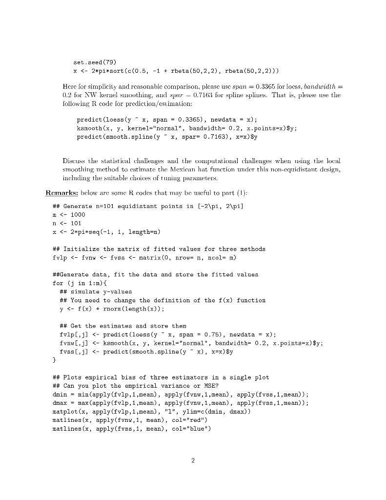
Step by Step Solution
There are 3 Steps involved in it
Step: 1

Get Instant Access to Expert-Tailored Solutions
See step-by-step solutions with expert insights and AI powered tools for academic success
Step: 2

Step: 3
Ace Your Homework with AI
Get the answers you need in no time with our AI-driven, step-by-step assistance
Get Started
Intermediate Business Analytics A Practical Approach To Descriptive Prescriptive And Predictive Analytics With R
Authors: Dr Yavuz Keceli
1st Edition
B0B4DR1J8G, 979-8837870552