it is an assigment and everything needs to be done!

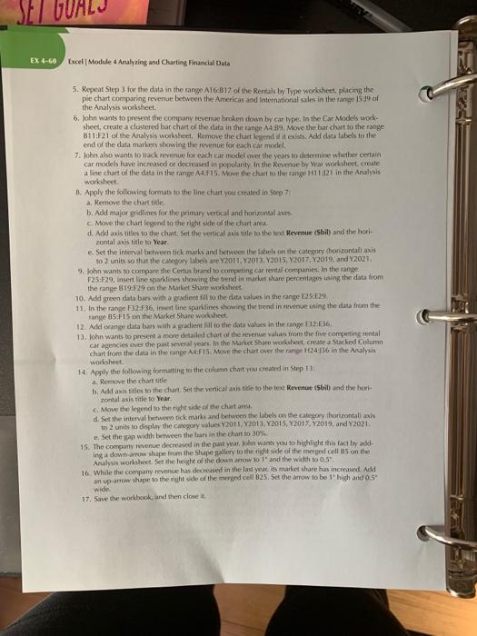
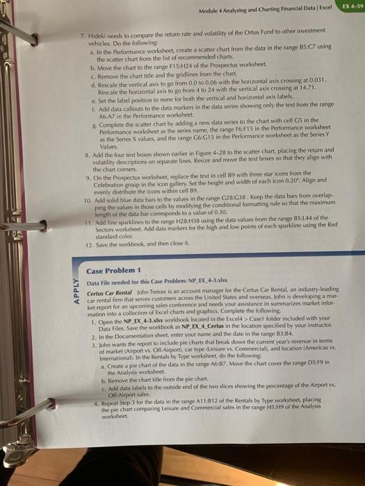
EX 4-60 Excel Module 4 Analyzing and Charting Financial 5. Repeat Step 3 for the data in the range A16B17 of the Rentak by Type worksheet, placing the pie chart comparing revenue between the Americas and International sales in the range 1519 of the Analysis worksheet 6. John wants to present the company revenue broken down by car type. In the Car Models work sheet, create a clustered bar chart of the data in the range A4 89. Move the bar churt to the range 811F21 of the Analysis worksheet. Remove the clart kigand it is easts. Add dies labels to the end of the data markers showing the revenue for each car model 7. John also wants to track revenue for each car model over the years to determine whether certain car models have increased or decreased in popularity. In the Revenue by Year worksheet, create a line chart of the data in the range A4.F15. Move the chart to the range H11.2 in the Analysis worksheet 8. Apply the following formats to the line chart you created in Step 7. 2 Remove the chart title b. Add major gridlines for the primary vertical and horizontalanes c. Move the chart legend to the right side of the chart are d. Add axis titles to the chart. Set the vertical axis title to the text Revenue (bit) and the hori zontal axis title to Year e. Set the interval between tick murks and between the fabels on the category horizontal axis to 2 units so that the category labels are 2011, 2013. Y2015. Y2017. Y2019, and Y2021 9. John wants to compare the Certus brand to competing car rental companies. In the range F25:F29, insert line sardines showing the trend in muru share percentages using the data from the range B19:29 on the Market share worksheet 10. Add green data bars with a gradient till to the data values in the range 025-29 11. In the range F32.736, mert line sparklines showing the trend in revenue using the data from the tange 5.F15 on the Market Slute worksheet 12. Add orange data burs with a gradient fill to the data values in the range 2:36 13. John wants to present a more detailed chart of the reverte values from the five competing rental car agencies over the past several years in the Market Share worksheet create a Stacked Column chart from the data in the range A4:15. Move the chart over the range H24956 in the Analysis worksheet 14. Apply the following formatting to the column chat you created in Step 13 a Remove the chart title b. Add axis titles to the chart. Set the vertical axistide to the text Revenue (bil) and the hori zontal axis title to Year Move the legend to the right side of the chartan d. Set the interval between tick marks and between the labels on the category horizontal axis to 2 units to display the category values 2011. 2013, 2015, 2017, Y2019, and Y2021 . Set the man with between the bars in the chart to 30% 15. The company revenue decreased in the past year. John wants you to highlight this fact by add Ing a down-arrow shape from the Shape gallery to the right side of the merged cells on the Analysis worksheet Set the height of the down to l' and the width to 0. 16. While the company revenue las decreased in the last year its market share has increased Add an up arrow shape to the right side of the med cell 825. Set the arrow to be 1 high and 0.5 wide 17. Save the workbook, and then close it EX 4-59 Module 4 Analyzing and Charting Financial Data Excel 7. Hidekl needs to compare the return rate and volatility of the Ortus Fund to other investment vehicles. Do the following: a. In the Performance worksheet, create a scatter chart from the data in the range B5:C7 using the scatter chart from the list of recommended charts. b. Move the chart to the range F15:H24 of the Prospectus worksheet. c. Remove the chart title and the gridlines from the chart d. Rescale the vertical axis to go from 0.0 to 0.06 with the horizontal axis crossing at 0.031. Rescate the horizontal axis to go from 4 to 24 with the vertical axis crossing at 14.71. e. Set the label position to none for both the vertical and horizontal axis labels. Add data callouts to the data markers in the data series showing only the text from the range A6A7 in the Performance worksheet. Complete the scatter chart by adding a new data series to the chart with cell G5 in the Performance worksheet as the series name, the range F6 F15 in the Performance worksheet as the Series X values, and the range G:G15 in the Performance worksheet as the Series Y Values 8. Add the four text boxes shown earlier in Figure 4-28 to the scatter chart, placing the return and volatility descriptions on separate lines. Resize and move the text boxes so that they align with the chart corners 9. On the Prospectus worksheet, replace the text in cell 89 with three star icons from the Celebration group in the icon gallery. Set the height and width of each icon 0.209. Align and evenly distribute the icons within cell 89. 10. Add solid blue data bars to the values in the range G28:G38. Keep the data bars from overlap- ping the values in those cells by modifying the conditional formatting rule so that the maximum length of the databar corresponds to a value of 0.30. 11. Add line sparklines to the range H28:38 using the data values from the range 85:144 of the Sectors worksheet. Add data markers for the high and low points of each sparkline using the Red standard color 12. Save the workbook, and then close it. APPLY Case Problem 1 Data File needed for this Case Problem: NP_EX_4-3.xlsx Certus Car Rental John Tretow is an account manager for the Certus Car Rental, an industry-leading car rental firm that serves customers across the United States and overseas. John is developing a mar- ket report for an upcoming sales conference and needs your assistance in marizes market indor mation into a collection of Excel charts and graphics. Complete the following 1. Open the NP_EX_4-3.xlsx workbook located in the Excel > Case folder included with your Data files. Save the workbook as NPEX_4_Certus in the location specified by your instructor 2. In the Documentation sheet, enter your name and the date in the range 33:34. 3. John wants the report to include pie charts that break down the current year's revenue in terms of market (Airport vs. Oll Airport, car type Leisure vs. Commerciall, and location (Americas vs. International. In the Rentals by Type worksheet, do the following: a. Create a pie chart of the data in the range A6:37. Move the chart cover the range D5F9 in the Analysis worksheet b. Remove the chart title from the pie chart c. Add data labels to the outside end of the two slices showing the percentage of the Airport vs Off Airport sales 4. Repeat Step 3 for the data in the range A11:B12 of the Rentals by Type worksheet placing the ple chart comparing Leisure and Commercial sales in the range HH9 of the Analysis worlasheet EX 4-60 Excel Module 4 Analyzing and Charting Financial 5. Repeat Step 3 for the data in the range A16B17 of the Rentak by Type worksheet, placing the pie chart comparing revenue between the Americas and International sales in the range 1519 of the Analysis worksheet 6. John wants to present the company revenue broken down by car type. In the Car Models work sheet, create a clustered bar chart of the data in the range A4 89. Move the bar churt to the range 811F21 of the Analysis worksheet. Remove the clart kigand it is easts. Add dies labels to the end of the data markers showing the revenue for each car model 7. John also wants to track revenue for each car model over the years to determine whether certain car models have increased or decreased in popularity. In the Revenue by Year worksheet, create a line chart of the data in the range A4.F15. Move the chart to the range H11.2 in the Analysis worksheet 8. Apply the following formats to the line chart you created in Step 7. 2 Remove the chart title b. Add major gridlines for the primary vertical and horizontalanes c. Move the chart legend to the right side of the chart are d. Add axis titles to the chart. Set the vertical axis title to the text Revenue (bit) and the hori zontal axis title to Year e. Set the interval between tick murks and between the fabels on the category horizontal axis to 2 units so that the category labels are 2011, 2013. Y2015. Y2017. Y2019, and Y2021 9. John wants to compare the Certus brand to competing car rental companies. In the range F25:F29, insert line sardines showing the trend in muru share percentages using the data from the range B19:29 on the Market share worksheet 10. Add green data bars with a gradient till to the data values in the range 025-29 11. In the range F32.736, mert line sparklines showing the trend in revenue using the data from the tange 5.F15 on the Market Slute worksheet 12. Add orange data burs with a gradient fill to the data values in the range 2:36 13. John wants to present a more detailed chart of the reverte values from the five competing rental car agencies over the past several years in the Market Share worksheet create a Stacked Column chart from the data in the range A4:15. Move the chart over the range H24956 in the Analysis worksheet 14. Apply the following formatting to the column chat you created in Step 13 a Remove the chart title b. Add axis titles to the chart. Set the vertical axistide to the text Revenue (bil) and the hori zontal axis title to Year Move the legend to the right side of the chartan d. Set the interval between tick marks and between the labels on the category horizontal axis to 2 units to display the category values 2011. 2013, 2015, 2017, Y2019, and Y2021 . Set the man with between the bars in the chart to 30% 15. The company revenue decreased in the past year. John wants you to highlight this fact by add Ing a down-arrow shape from the Shape gallery to the right side of the merged cells on the Analysis worksheet Set the height of the down to l' and the width to 0. 16. While the company revenue las decreased in the last year its market share has increased Add an up arrow shape to the right side of the med cell 825. Set the arrow to be 1 high and 0.5 wide 17. Save the workbook, and then close it EX 4-59 Module 4 Analyzing and Charting Financial Data Excel 7. Hidekl needs to compare the return rate and volatility of the Ortus Fund to other investment vehicles. Do the following: a. In the Performance worksheet, create a scatter chart from the data in the range B5:C7 using the scatter chart from the list of recommended charts. b. Move the chart to the range F15:H24 of the Prospectus worksheet. c. Remove the chart title and the gridlines from the chart d. Rescale the vertical axis to go from 0.0 to 0.06 with the horizontal axis crossing at 0.031. Rescate the horizontal axis to go from 4 to 24 with the vertical axis crossing at 14.71. e. Set the label position to none for both the vertical and horizontal axis labels. Add data callouts to the data markers in the data series showing only the text from the range A6A7 in the Performance worksheet. Complete the scatter chart by adding a new data series to the chart with cell G5 in the Performance worksheet as the series name, the range F6 F15 in the Performance worksheet as the Series X values, and the range G:G15 in the Performance worksheet as the Series Y Values 8. Add the four text boxes shown earlier in Figure 4-28 to the scatter chart, placing the return and volatility descriptions on separate lines. Resize and move the text boxes so that they align with the chart corners 9. On the Prospectus worksheet, replace the text in cell 89 with three star icons from the Celebration group in the icon gallery. Set the height and width of each icon 0.209. Align and evenly distribute the icons within cell 89. 10. Add solid blue data bars to the values in the range G28:G38. Keep the data bars from overlap- ping the values in those cells by modifying the conditional formatting rule so that the maximum length of the databar corresponds to a value of 0.30. 11. Add line sparklines to the range H28:38 using the data values from the range 85:144 of the Sectors worksheet. Add data markers for the high and low points of each sparkline using the Red standard color 12. Save the workbook, and then close it. APPLY Case Problem 1 Data File needed for this Case Problem: NP_EX_4-3.xlsx Certus Car Rental John Tretow is an account manager for the Certus Car Rental, an industry-leading car rental firm that serves customers across the United States and overseas. John is developing a mar- ket report for an upcoming sales conference and needs your assistance in marizes market indor mation into a collection of Excel charts and graphics. Complete the following 1. Open the NP_EX_4-3.xlsx workbook located in the Excel > Case folder included with your Data files. Save the workbook as NPEX_4_Certus in the location specified by your instructor 2. In the Documentation sheet, enter your name and the date in the range 33:34. 3. John wants the report to include pie charts that break down the current year's revenue in terms of market (Airport vs. Oll Airport, car type Leisure vs. Commerciall, and location (Americas vs. International. In the Rentals by Type worksheet, do the following: a. Create a pie chart of the data in the range A6:37. Move the chart cover the range D5F9 in the Analysis worksheet b. Remove the chart title from the pie chart c. Add data labels to the outside end of the two slices showing the percentage of the Airport vs Off Airport sales 4. Repeat Step 3 for the data in the range A11:B12 of the Rentals by Type worksheet placing the ple chart comparing Leisure and Commercial sales in the range HH9 of the Analysis worlasheet