It seems very long but it only takes 5 minutes, please help me.

using Matlab to solve.

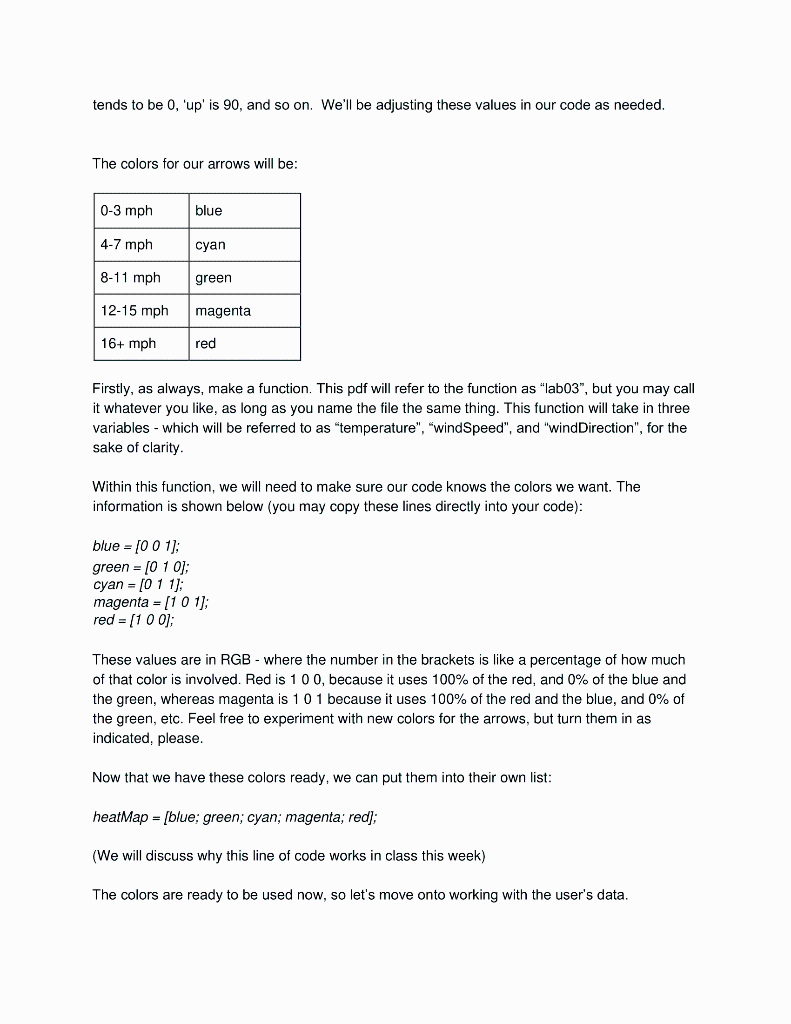
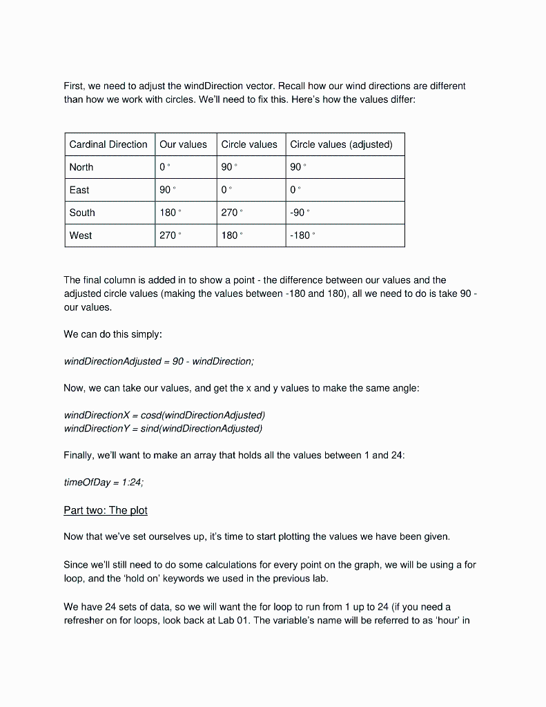
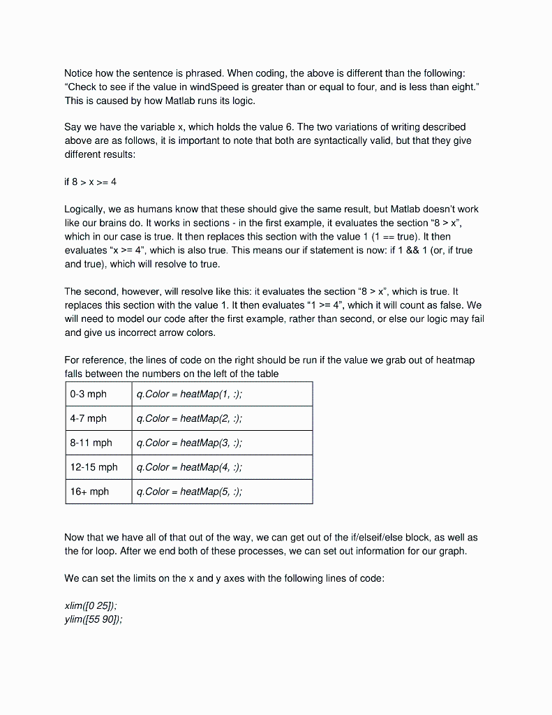
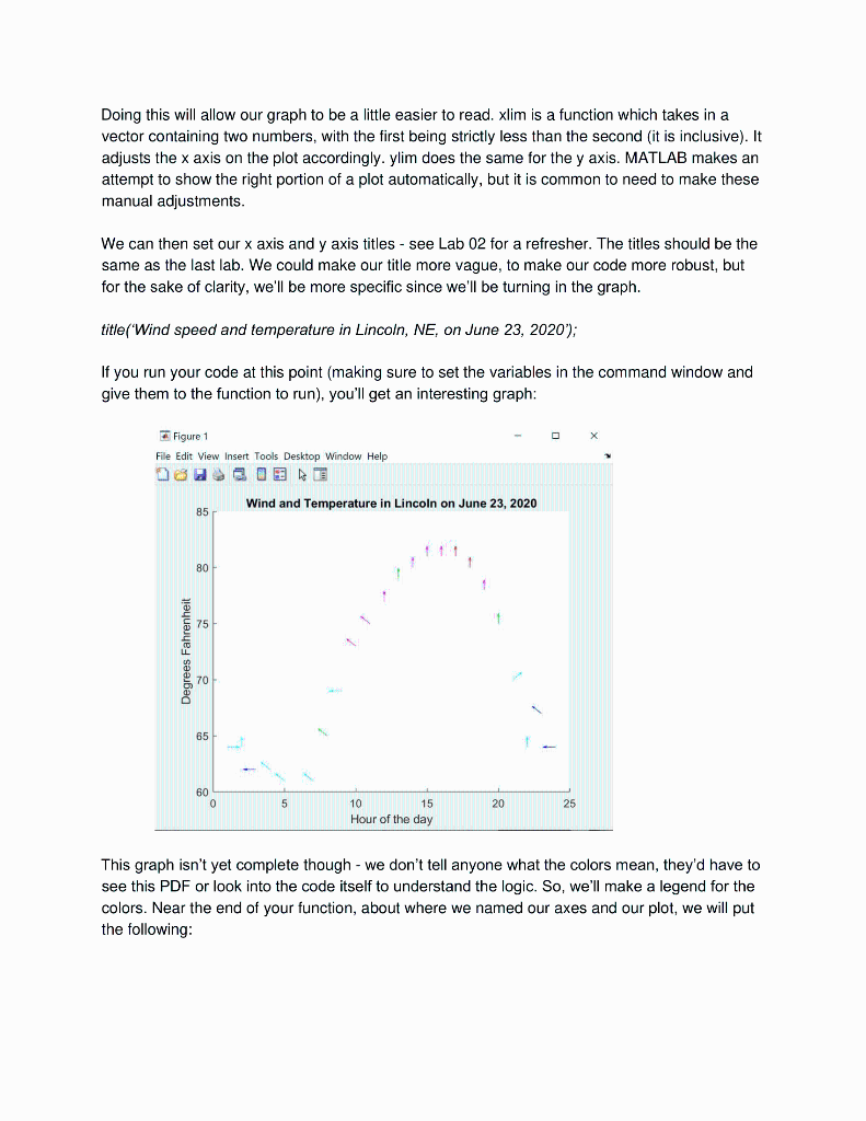
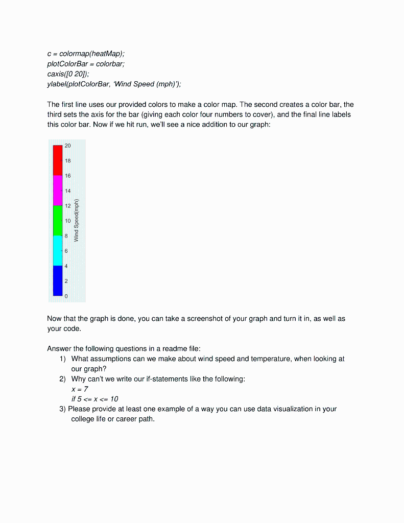
Combined Temperature, Windspeed, and Direction Plot Goal: Plot temperature, wind speed, and direction with increasing time of day. You Should Turn In Item 1: Final graph plot of Lincoln, North Platte, and Grand Island as a JPG or PNG file Item 2: Your code, as a .m file Item 3: A readme file, answering the questions at the end of the lab. Our code, and what it will do: Part one: The setup In the previous lab, we took information from the user - 2 sets of data, each containing 24 temperatures, as well as a string saying when the data was collected - and turned it into a graph. In this lab, we will take in a total of 3 sets of data - temperatures from a city over a 24 hour period, as well as the wind speed and wind direction. What we will do with this data is make a plot, where the points on the plot are the temperature at a certain time of day. From these dots, there will be arrows pointing in the direction of the wind at that time, and the color of the arrows will show how strong the wind was. Here are our values: Temperatures: [64 64 62 62 61 57 61 65 69 73 75 77 79 80 81 81 81 80 78 75 70 64 67 64] Wind speed: [6 73 6 606 85 12 15 14 8 14 14 15 17 18 15 8 7 6 3 3] Wind direction: [90 0 270 315 3150 315 315 270 315 315 0 0 0 0 0 0 0 0 0 45 0 315 270) Note: The numbers under "wind direction" assume that is North, 90 is East, 180 is South, and 270 is West. Since we'll be associating 'up' with North, 'right' with East and so forth, this means there is a disconnect between our numbers and how we work with circles in math - as 'right' tends to be 0, 'up' is 90, and so on. We'll be adjusting these values in our code as needed. The colors for our arrows will be: 0-3 mph blue 4-7 mph cyan 8-11 mph green 12-15 mph magenta 16+ mph red Firstly, as always, make a function. This pdf will refer to the function as lab03", but you may call it whatever you like, as long as you name the file the same thing. This function will take in three variables - which will be referred to as "temperature", "windSpeed", and "wind Direction", for the sake of clarity. Within this function, we will need to make sure our code knows the colors we want. The information is shown below (you may copy these lines directly into your code): blue = 10 0 1]; green = {0 1 0); cyan = 011; magenta = [1 0 1); red = (1 0 0]; These values are in RGB - where the number in the brackets is like a percentage of how much of that color is involved. Red is 100, because it uses 100% of the red, and 0% of the blue and the green, whereas magenta is 10 because it uses 100% of the red and the blue, and 0% of the green, etc. Feel free to experiment with new colors for the arrows, but turn them in as indicated, please. Now that we have these colors ready, we can put them into their own list: heatMap = [blue, green; cyan; magenta; red); (We will discuss why this line of code works in class this week) The colors are ready to be used now, so let's move onto working with the user's data. First, we need to adjust the wind Direction vector. Recall how our wind directions are different than how we work with circles. We'll need to fix this. Here's how the values differ: Cardinal Direction Our values Circle values Circle values (adjusted) North 0 90 90 East 90 0 0 South 180 270 -90 West 270 180 -180 The final column is added in to show a point - the difference between our values and the adjusted circle values (making the values between - 180 and 180), all we need to do is take 90 - our values. We can do this simply: windDirection Adjusted = 90 - wind Direction; Now, we can take our values, and get the x and y values to make the same angle: windDirectionX = cos(wind Direction Adjusted) windDirection Y = sind(wind Direction Adjusted) Finally, we'll want to make an array that holds all the values between 1 and 24: timeOfDay = 1:24: Part two: The plot Now that we've set ourselves up, it's time to start plotting the values we have been given. Since we'll still need to do some calculations for every point on the graph, we will be using a for loop, and the 'hold on' keywords we used in the previous lab. We have 24 sets of data, so we will want the for loop to run from 1 up to 24 (if you need a refresher on for loops, look back at Lab 01. The variable's name will be referred to as 'hour' in this lab). We want the graph to take in all of our data, so right after starting the loop we will tell the plot to hold on. Now, we will be learning about a new function: Quiver. Quiver is a function that will allow us to make our points on the graph into arrows. It takes in four values: the x value of the plot, the y value of the plot, the x value of the arrow length, and the y value of the arrow height. We already have all these values, from before we started the for loop, so we just need to give them to quiver. 9 = quiver(timeOfDay(hour), temperature/hour), wind DirectionX(hour), wind Direction Y/hour)); Note one: Since all of our variables show (timeOfDay, temperature, wind Direction X, windDirection Y) are all lists of numbers, and we're stepping through them one value at a time, we need to specify which number we want out of them. Since 'hour' is going from 1 to 24 over the course of the for loop, we can grab the first value, then the second value, etc, all the way to the 24th value within these lists. Note two: notice we are making a new variable 'q' here - it holds the information for our point on the graph. We need to keep track of this since we still wish to adjust the information. After creating the point, we want to make sure the arrows aren't too big: q. Max HeadSize = 1; This line will make sure the arrow head size is appropriate to our graph. Next, we will need to associate the arrow with a color. Recall the values we wish the colors to correspond to (top of page 2). This will require an if/elseif/else block. A hint on how to work with the if/elseif/else block: Start with checking all values less than (and not equal to) four. We will be comparing the separate values within the wind Speed variable, like how we grabbed specific values from other arrays when using the quiver function. If the number we grabbed out of wind Speed is strictly smaller than four, we will run the following code: q.Color = heatMap(1, :); Next, we will check to see if the value in wind Speed is greater than or equal to four, and that the value in wind Speed is strictly less than eight. Notice how the sentence is phrased. When coding, the above is different than the following: "Check to see if the value in wind Speed is greater than or equal to four, and is less than eight." This is caused by how Matlab runs its logic. Say we have the variable x, which holds the value 6. The two variations of writing described above are as follows, it is important to note that both are syntactically valid, but that they give different results: if 8 > X >= 4 Logically, we as humans know that these should give the same result, but Matlab doesn't work like our brains do. It works in sections - in the first example, it evaluates the section "8 >x", which in our case is true. It then replaces this section with the value 1 (1 == true). It then evaluates "x >= 4", which is also true. This means our if statement is now: if 1 && 1 (or, if true and true), which will resolve to true. The second, however, will resolve like this: it evaluates the section "8 > x", which is true. It replaces this section with the value 1. It then evaluates "1 >= 4", which it will count as false. We will need to model our code after the first example, rather than second, or else our logic may fail and give us incorrect arrow colors. For reference, the lines of code on the right should be run if the value we grab out of heatmap falls between the numbers on the left of the table 0-3 mph q. Color = heatmap(1. :); 4-7 mph q.Color = heatmap(2, :); 8-11 mph q. Color = heatMap(3. :); 12-15 mph q. Color - heatMap(4, :); 16+ mph q. Color = heatmap(5, :); Now that we have all of that out of the way, we can get out of the if/elseif/else block, as well as the for loop. After we end both of these processes, we can set out information for our graph. We can set the limits on the x and y axes with the following lines of code: xlim ([025]); ylim (55 90]); Doing this will allow our graph to be a little easier to read. xlim is a function which takes in a vector containing two numbers, with the first being strictly less than the second (it is inclusive). It adjusts the x axis on the plot accordingly. ylim does the same for the y axis. MATLAB makes an attempt to show the right portion of a plot automatically, but it is common to need to make these manual adjustments. We can then set our x axis and y axis titles - see Lab 02 for a refresher. The titles should be the same as the last lab. We could make our title more vague, to make our code more robust, but for the sake of clarity, we'll be more specific since we'll be turning in the graph. title('Wind speed and temperature in Lincoln, NE, on June 23, 2020'); If you run your code at this point (making sure to set the variables in the command window and give them to the function to run), you'll get an interesting graph: Figure 1 File Edit View Insert Tools Desktop Window Help OBIEKT Wind and Temperature Lincoln on June 23, 2020 85 80 75 Degrees Fahrenheit 65 60 0 5 20 25 10 15 Hour of the day This graph isn't yet complete though - we don't tell anyone what the colors mean, they'd have to see this PDF or look into the code itself to understand the logic. So, we'll make a legend for the colors. Near the end of your function, about where we named our axes and our plot, we will put the following: C = colormap/heatMap); plotColorBar = colorbar; caxis([020]); ylabel(plotColorBar, 'Wind Speed (mph)); The first line uses our provided colors to make a color map. The second creates a color bar, the third sets the axis for the bar (giving each color four numbers to cover), and the final line labels this color bar. Now if we hit run, we'll see a nice addition to our graph: 20 18 16 14 12 10 Wind Speed (mph) 6 4 2 0 Now that the graph is done, you can take a screenshot of your graph and turn it in, as well as your code Answer the following questions in a readme file: 1) What assumptions can we make about wind speed and temperature, when looking at our graph? 2) Why can't we write our if-statements like the following: X = 7 if 5 X >= 4 Logically, we as humans know that these should give the same result, but Matlab doesn't work like our brains do. It works in sections - in the first example, it evaluates the section "8 >x", which in our case is true. It then replaces this section with the value 1 (1 == true). It then evaluates "x >= 4", which is also true. This means our if statement is now: if 1 && 1 (or, if true and true), which will resolve to true. The second, however, will resolve like this: it evaluates the section "8 > x", which is true. It replaces this section with the value 1. It then evaluates "1 >= 4", which it will count as false. We will need to model our code after the first example, rather than second, or else our logic may fail and give us incorrect arrow colors. For reference, the lines of code on the right should be run if the value we grab out of heatmap falls between the numbers on the left of the table 0-3 mph q. Color = heatmap(1. :); 4-7 mph q.Color = heatmap(2, :); 8-11 mph q. Color = heatMap(3. :); 12-15 mph q. Color - heatMap(4, :); 16+ mph q. Color = heatmap(5, :); Now that we have all of that out of the way, we can get out of the if/elseif/else block, as well as the for loop. After we end both of these processes, we can set out information for our graph. We can set the limits on the x and y axes with the following lines of code: xlim ([025]); ylim (55 90]); Doing this will allow our graph to be a little easier to read. xlim is a function which takes in a vector containing two numbers, with the first being strictly less than the second (it is inclusive). It adjusts the x axis on the plot accordingly. ylim does the same for the y axis. MATLAB makes an attempt to show the right portion of a plot automatically, but it is common to need to make these manual adjustments. We can then set our x axis and y axis titles - see Lab 02 for a refresher. The titles should be the same as the last lab. We could make our title more vague, to make our code more robust, but for the sake of clarity, we'll be more specific since we'll be turning in the graph. title('Wind speed and temperature in Lincoln, NE, on June 23, 2020'); If you run your code at this point (making sure to set the variables in the command window and give them to the function to run), you'll get an interesting graph: Figure 1 File Edit View Insert Tools Desktop Window Help OBIEKT Wind and Temperature Lincoln on June 23, 2020 85 80 75 Degrees Fahrenheit 65 60 0 5 20 25 10 15 Hour of the day This graph isn't yet complete though - we don't tell anyone what the colors mean, they'd have to see this PDF or look into the code itself to understand the logic. So, we'll make a legend for the colors. Near the end of your function, about where we named our axes and our plot, we will put the following: C = colormap/heatMap); plotColorBar = colorbar; caxis([020]); ylabel(plotColorBar, 'Wind Speed (mph)); The first line uses our provided colors to make a color map. The second creates a color bar, the third sets the axis for the bar (giving each color four numbers to cover), and the final line labels this color bar. Now if we hit run, we'll see a nice addition to our graph: 20 18 16 14 12 10 Wind Speed (mph) 6 4 2 0 Now that the graph is done, you can take a screenshot of your graph and turn it in, as well as your code Answer the following questions in a readme file: 1) What assumptions can we make about wind speed and temperature, when looking at our graph? 2) Why can't we write our if-statements like the following: X = 7 if 5