

it the last picture is the first question, and the second to last is the second question and so on
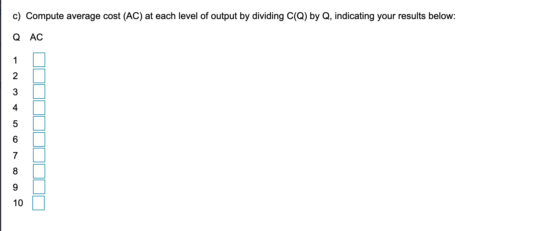
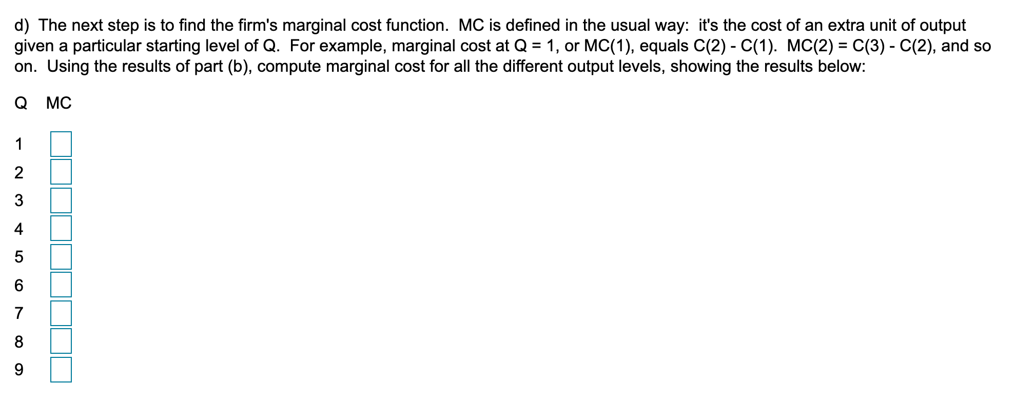
Suppose a rm uses capital (K) and labor (L) to produce widgets according to the production function Q = K1'4L1'4 = (KL)1'4, where Q is output. The goal in this problem is to nd the rm's total and marginal cost functions. In order to derive the cost function, the first step is to nd the location of the cost-minimizing bundle on any given isoquant. To get a numerical answer, recall that the slope of an isoquant is -MP|_/MPK (K is on the vertical axis). Using calculus, it can be shown that this slope formula reduces to -K/L. For example, consider the input bundle with K = 8, L = 2 on the isoquant with Q = 2 (note that 2 = 16\"4 ). The formula indicates that the slope at this point is -4 = -8/2. In fact, the formula tells us that regardless of which isoquant an input bundle is on, the slope will be -4 as long as the ratio of K to L is 4:1. Similarly, the isoquant slope will be -1 whenever the ratio of K to L is 1:1. In answering the following questions, use integer values only (don't enter unneeded decimal points). a) Suppose that the wage is $2 per hour and that capital also rents for $2 per hour. The slope of the isocost line is than equal to negative D. Using resulting slope value along with the above formula for the isoquant slope, compute the firm's optimal input ratio at any cost-minimizing point (recall that the isoquant and isocost slopes are equal at a tangency point). This ratio is (enter a single integer). Now suppose that the rm wants to produce one widget (Q = 1). Using your previous result on the optimal input ratio, you can compute the input levels that the rm uses to produce this output. These levels are K = D and L = D. The cost of this input bundle is $El, which gives cm (the cost function C(Q) evaluated at Q=1). b) The cost-minimizing input bundle when Q = 2 has K = I: and L = . The cost of this bundle is , which gives 0(2). b) The cost-minimizing input bundle when Q = 2 has K = D and L = D. The cost of this bundle is D, which gives 0(2). 0) Repeat this calculation for Q = 2,3,...,10, indicating your results below: Q K L C(Q) | | |_l__|_l__|_l |_l__|_l__|_l c) Compute average cost (AC) at each level of output by dividing C(Q) by Q, indicating your results below: Q AC 2 CO 00 - ) OF A W 10d) The next step is to find the firm's marginal cost function. MC is defined in the usual way: it's the cost of an extra unit of output given a particular starting level of Q. For example, marginal cost at Q = 1, or MC(1), equals C(2) - C(1). MC(2) = C(3) - C(2), and so on. Using the results of part (b), compute marginal cost for all the different output levels, showing the results below: Q MC 10 00 ~ ) UI A W N6) On a piece of paper. graph both the MC and AC functions. They are 0 A. convex, upward sloping curves 0 B. upward-sloping straight lines 0 c. Ushaped curves 0 D. horizontal lines


