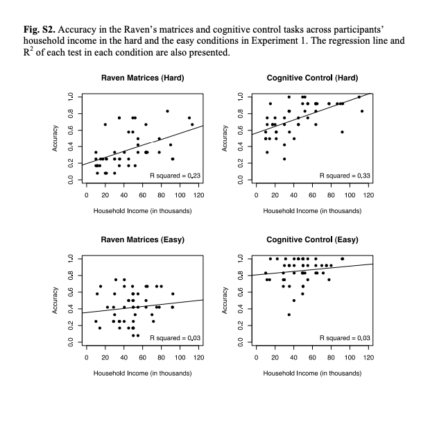
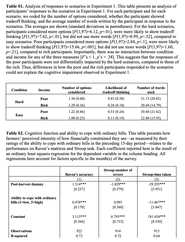
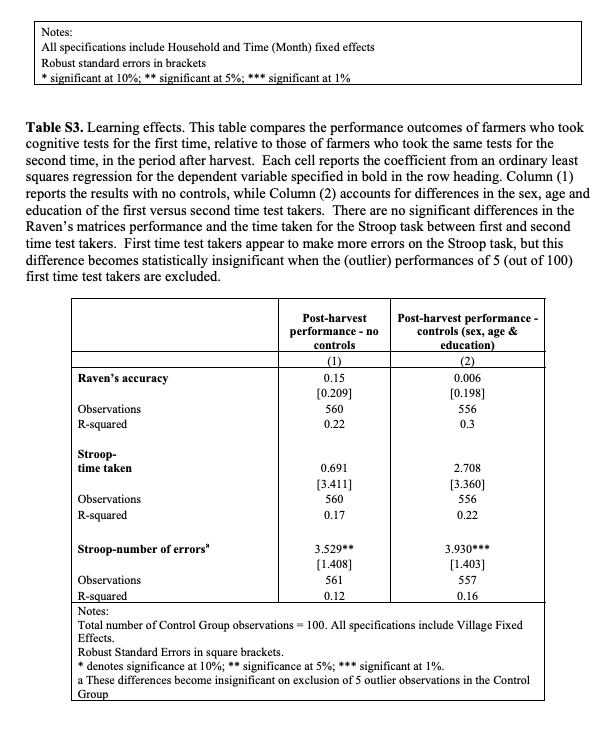
IT WOULD MEAN THE WORLD TO ME IF YOU COULD ANSWER THESE QUESTIONS WITHIN 12HRS. The question and the supplements have been attached. I have been a course hero member for a long time, and i have never before needed this service as much as i do now. Hope you can deliver.

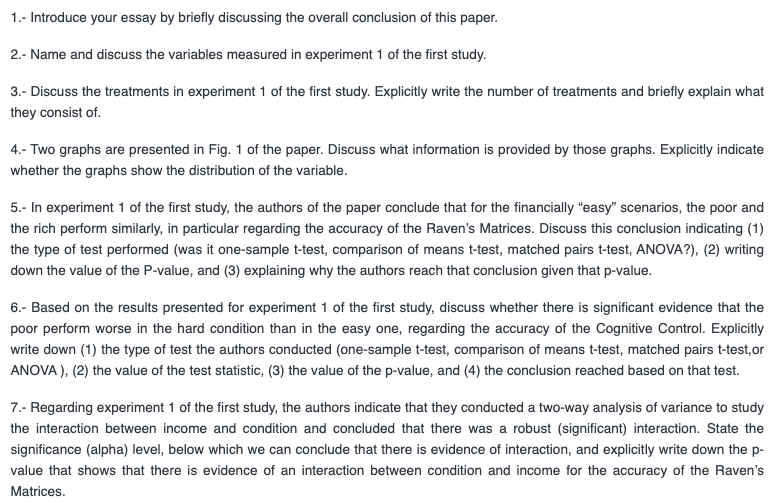
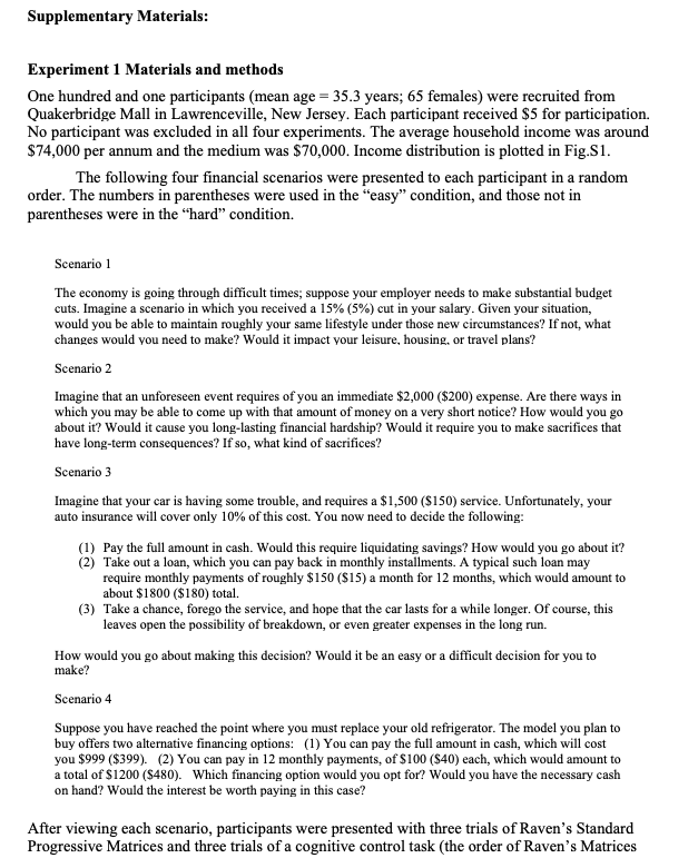
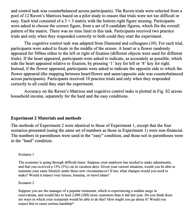
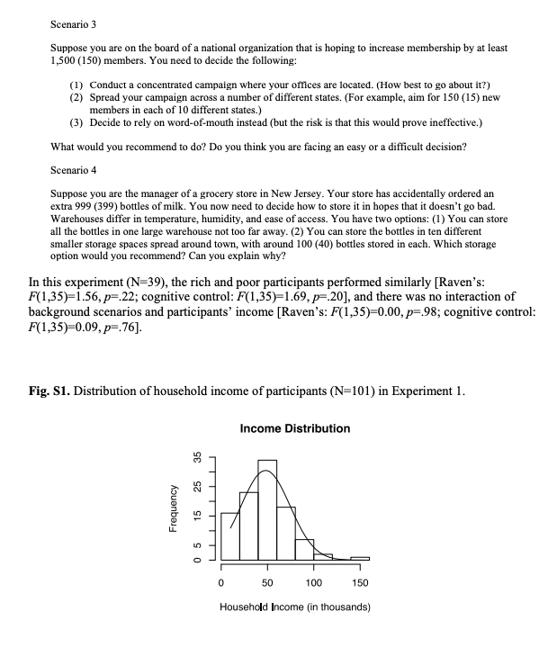
1.- Introduce your essay by briefly discussing the overall conclusion of this paper. 2.- Name and discuss the variables measured in experiment1 of the first study. 3. Discuss the treatments in experiment 1 of the first study. Explicitly write the number of treatments and briefly explain what they consist of. 4.- Two graphs are presented in Fig. 1 of the paper. Discuss what information is provided by those graphs. Explicitly indicate whether the graphs show the distribution of the variable. 5.- In experiment 1 of the first study, the authors of the paper conclude that for the financially \"easy\" scenarios, the poor and the rich perform similarly, in particular regarding the accuracy of the Flaven's Matrices. Discuss this conclusion indicating [1] the type of test performed {was it one-sample t-test, comparison of means t-test, matched pairs t-test, ANGvA't]. {2] writing down the value at the F-vatue, and {3} explaining why the authors reach that conelusien given that tit-value. e.- Based on the results presented for experiment 1 of the rst study. discuss whether there is significant evidence that the poor perform worse in the hard condition than in the easy one, regarding the accuracy of the Cognitive Control. Explicitly write down [1] the type of test the authors conducted [one-sample t-test. comparison of means t-test, matched pairs t-test.or move 1, [2] the value of the test statistic, [3} the value of the p-value, and {4} the conclusion reached based on that test. ?.- Ftegarding experiment 1 of the first study, the authors indicate that they conducted a two-way analysis of variance to study the interaction bemeen income and condition and concluded that there was a robust [signicant] interaction. State the significance {alpha} level, below which we can conclude that there is evidence of interaction. and explicitly write down the p- value that shows that there is evidence of an interaction bemeen condition and income for the accuracy of the Flaven's Matrices. Supplementary Materials: Experiment 1 Materials and methods One hundred and one participants (mean age = 35.3 years; 65 females) were recruited from Quakerbridge Mall in Lawrenceville, New Jersey. Each participant received $5 for participation. No participant was excluded in all four experiments. The average household income was around $74,000 per annum and the medium was $70,000. Income distribution is plotted in Fig.$1. The following four financial scenarios were presented to each participant in a random order. The numbers in parentheses were used in the "easy" condition, and those not in parentheses were in the "hard" condition. Scenario 1 The economy is going through difficult times; suppose your employer needs to make substantial budget cuts. Imagine a scenario in which you received a 15% (5%) cut in your salary. Given your situation, would you be able to maintain roughly your same lifestyle under those new circumstances? If not, what changes would you need to make? Would it impact your leisure, housing. or travel plans? Scenario 2 Imagine that an unforeseen event requires of you an immediate $2,000 ($200) expense. Are there ways in which you may be able to come up with that amount of money on a very short notice? How would you go about it? Would it cause you long-lasting financial hardship? Would it require you to make sacrifices that have long-term consequences? If so, what kind of sacrifices? Scenario 3 Imagine that your car is having some trouble, and requires a $1,500 ($150) service. Unfortunately, your auto insurance will cover only 10% of this cost. You now need to decide the following: (1) Pay the full amount in cash. Would this require liquidating savings? How would you go about it? (2) Take out a loan, which you can pay back in monthly installments. A typical such loan may require monthly payments of roughly $150 ($15) a month for 12 months, which would amount to about $1800 ($180) total. (3) Take a chance, forego the service, and hope that the car lasts for a while longer. Of course, this leaves open the possibility of breakdown, or even greater expenses in the long run. How would you go about making this decision? Would it be an easy or a difficult decision for you to make? Scenario 4 Suppose you have reached the point where you must replace your old refrigerator. The model you plan to buy offers two alternative financing options: (1) You can pay the full amount in cash, which will cost you $999 ($399). (2) You can pay in 12 monthly payments, of $100 ($40) each, which would amount to a total of $1200 ($480). Which financing option would you opt for? Would you have the necessary cash on hand? Would the interest be worth paying in this case? After viewing each scenario, participants were presented with three trials of Raven's Standard Progressive Matrices and three trials of a cognitive control task (the order of Raven's Matricesand control task was counterbalanced across participants). The Raven trials were selected from a pool of 12 Raven's Matrices based on a pilot study to ensure that trials were not too difficult or easy. Each trial consisted of a 3 x 3 matrix with the bottom right figure missing. Participants were asked to choose the correct figure, from a set of 8 candidate figures, which fits the overall pattern of the matrix. There was no time limit in this task. Participants received two practice trials and only when they responded correctly to both could they start the experiment. The cognitive control task was adapted from Diamond and colleagues (30). For each trial, participants were asked to fixate in the middle of the screen. A heart or a flower randomly appeared for 500ms either to the left or right of fixation (different objects were used for different trials). If the heart appeared, participants were asked to indicate, as accurately as possible, which side the heart appeared relative to fixation, by pressing '1' key for left or '8' key for right. Instead, if the flower appeared, participants were asked to indicate the opposite side to which the flower appeared (the mapping between heart/flower and same/opposite side was counterbalanced across participants). Participants received 10 practice trials and only when they responded correctly to all could they start the experiment. Accuracy on the Raven's Matrices and cognitive control tasks is plotted in Fig. $2 across household income, separately for the hard and the easy conditions. Experiment 2 Materials and methods The methods of Experiment 2 were identical to those of Experiment 1, except that the four scenarios presented (using the same set of numbers as those in Experiment 1) were non-financial. The numbers in parentheses were used in the "easy" condition, and those not in parentheses were in the "hard" condition. Scenario 1 The economy is going through difficult times. Suppose your employer has needed to make adjustments, and that you received a 15% (5%) cut in vacation days. Given your current situation, would you be able to maintain your same lifestyle under those new circumstances? If not, what changes would you need to make? Would it impact your leisure, housing, or travel plans? Scenario 2 Suppose you are the manager of a popular restaurant, which is experiencing a sudden surge in reservations, and would like to feed 2,000 (200) more customers than it did last year. Do you think there are ways in which your restaurant would be able to do this? How might you go about it? Would you expect this to cause serious hardship?Scenario 3 Suppose you are on the board of a national organization that is hoping to increase membership by at least 1,500 (150) members. You need to decide the following: (1) Conduct a concentrated campaign where your offices are located. (How best to go about it?) (2) Spread your campaign across a number of different states. (For example, aim for 150 (15) new members in each of 10 different states.) (3) Decide to rely on word-of-mouth instead (but the risk is that this would prove ineffective.) What would you recommend to do? Do you think you are facing an easy or a difficult decision? Scenario 4 Suppose you are the manager of a grocery store in New Jersey. Your store has accidentally ordered an extra 999 (399) bottles of milk. You now need to decide how to store it in hopes that it doesn't go bad. Warehouses differ in temperature, humidity, and ease of access. You have two options: (1) You can store all the bottles in one large warehouse not too far away. (2) You can store the bottles in ten different smaller storage spaces spread around town, with around 100 (40) bottles stored in each. Which storage option would you recommend? Can you explain why? In this experiment (N=39), the rich and poor participants performed similarly [Raven's: F(1,35)=1.56, p=.22; cognitive control: F(1,35)=1.69, p=.20], and there was no interaction of background scenarios and participants' income [Raven's: F(1,35)=0.00, p=.98; cognitive control: F(1,35)=0.09, p=.76]. Fig. S1. Distribution of household income of participants (N=101) in Experiment 1. Income Distribution Frequency 15 0 5 0 50 100 150 Household Income (in thousands)Fig. $2. Accuracy in the Raven's matrices and cognitive control tasks across participants' household income in the hard and the easy conditions in Experiment 1. The regression line and R of each test in each condition are also presented. Raven Matrices (Hard) Cognitive Control (Hard) Accuracy 0.0 0.2 0.4 0.6 0.8 1.0 Accuracy A squared = 0.23 0.0 0.2 0.4 0.6 0.8 1.0 R squared = 0,33 0 20 40 60 80 100 120 0 20 40 60 80 100 120 Household Income (in thousands) Household Income (in thousands) Raven Matrices (Easy) Cognitive Control (Easy) Accuracy 0.0 0.2 0.4 0.6 0.8 1.0 Accuracy A squared = 0.03 0.0 0.2 0.4 0.6 0.8 1.0 R squared = 0,03 0 20 40 60 80 100 120 0 20 40 60 80 100 120 Household Income (in thousands) Household Income (in thousands)Table S1. Analysis of responses to scenarios in Experiment 1. This table presents an analysis of participants' responses to the scenarios in Experiment 1. For each participant and for each scenario, we coded for the number of options considered, whether the participant showed tradeoff thinking, and the average number of words written by the participant in response to the scenarios. The averages are shown (standard deviations in parentheses). For the hard scenarios participants considered more options [F(1,97)-6.12, p=.01], were more likely to show tradeoff thinking [F(1,97)=7.62, p<.01 but did not use more words p=".32]," compared to easy scenarios. poor participants considered options were likely show tradeoff thinking rich participants. importantly there was no interaction between condition and income for any of the three measures> .38]. This suggests that the responses of the poor participants were not differentially impacted by the hard scenarios, compared to those of the rich. Thus, differences in how the poor and the rich participants responded to the scenarios could not explain the cognitive impairment observed in Experiment 1. Condition Income Number of options Likelihood of Number of words considered tradeoff thinking used Hard Poor 1.36 (0.60) 0.43 (0.28) 31.13 (20.82) Rich 1.29 (0.36) 0.28 (0.18) 29.69 (14.79) Poor Easy 1.22 (0.46) 0.33 (0.24) 30.60 (21.62) Rich 1.00 (0.25) 0.13 (0.19) 22.88 (15.95) Table S2. Cognitive function and ability to cope with ordinary bills. This table presents how farmers' perceived intensity of how financially constrained they are-as measured by their ratings of the ability to cope with ordinary bills in the preceding 15-day period-relates to the performance on Raven's matrices and Stroop task. Each coefficient reported here is the result of an ordinary least squares regression for the dependent variable in the column heading. All regressions here account for factors specific to the month(s) of the survey. Stroop-number of Raven's accuracy errors Stroop-time taken (1) (2) (3) Post-harvest dummy 1.314+ 1.829* * * 29.295* [0.257] [0.579] [5.951] Ability to cope with ordinary bills (1=low, 3-high) 0.478* 0.093 -11.467** * [0.170] [0.360] [3.847] Constant 3.115* *# 6.793* * * 181.438* * * [0.366] [0.733] [8.550] Observations 922 914 913 R-squared 0.72 0.72 0.66Notes: All specifications include Household and Time (Month) fixed effects Robust standard errors in brackets * significant at 10%; ** significant at 5%; * significant at 1% Table S3. Learning effects. This table compares the performance outcomes of farmers who took cognitive tests for the first time, relative to those of farmers who took the same tests for the second time, in the period after harvest. Each cell reports the coefficient from an ordinary least squares regression for the dependent variable specified in bold in the row heading. Column (1) reports the results with no controls, while Column (2) accounts for differences in the sex, age and education of the first versus second time test takers. There are no significant differences in the Raven's matrices performance and the time taken for the Stroop task between first and second time test takers. First time test takers appear to make more errors on the Stroop task, but this difference becomes statistically insignificant when the (outlier) performances of 5 (out of 100) first time test takers are excluded. Post-harvest Post-harvest performance - performance - no controls (sex, age & controls education) (1) (2) Raven's accuracy D.15 0.006 [0.209] [0.198] Observations 560 556 R-squared 0.22 0.3 Stroop- time taken 0.691 2.708 [3.411] (3.360] Observations 560 556 R-squared 0.17 0.22 Stroop-number of errors" 3.529- 3.930* *. [1.408] [1.403] Observations 561 557 R-squared 0.12 0.16 Notes: Total number of Control Group observations = 100. All specifications include Village Fixed Effects. Robust Standard Errors in square brackets. * denotes significance at 10%; "* significance at 5%; *** significant at 1%. a These differences become insignificant on exclusion of 5 outlier observations in the Control Group