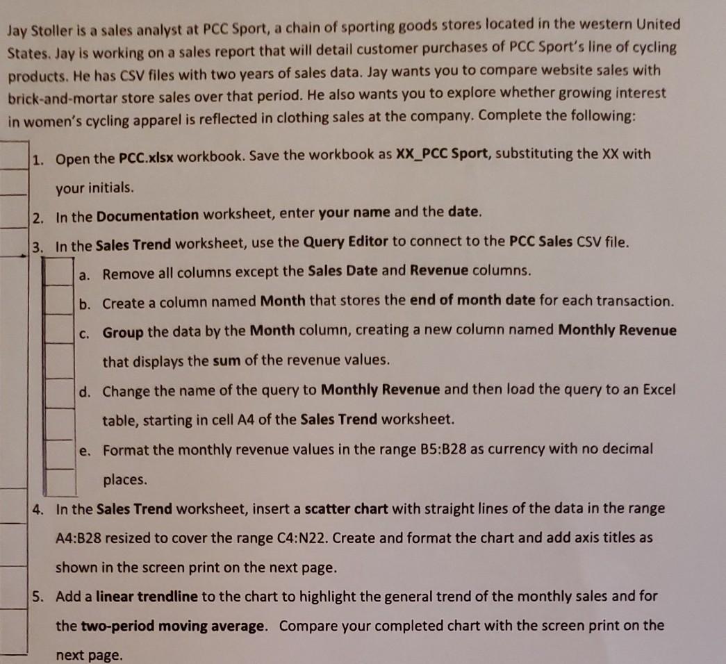
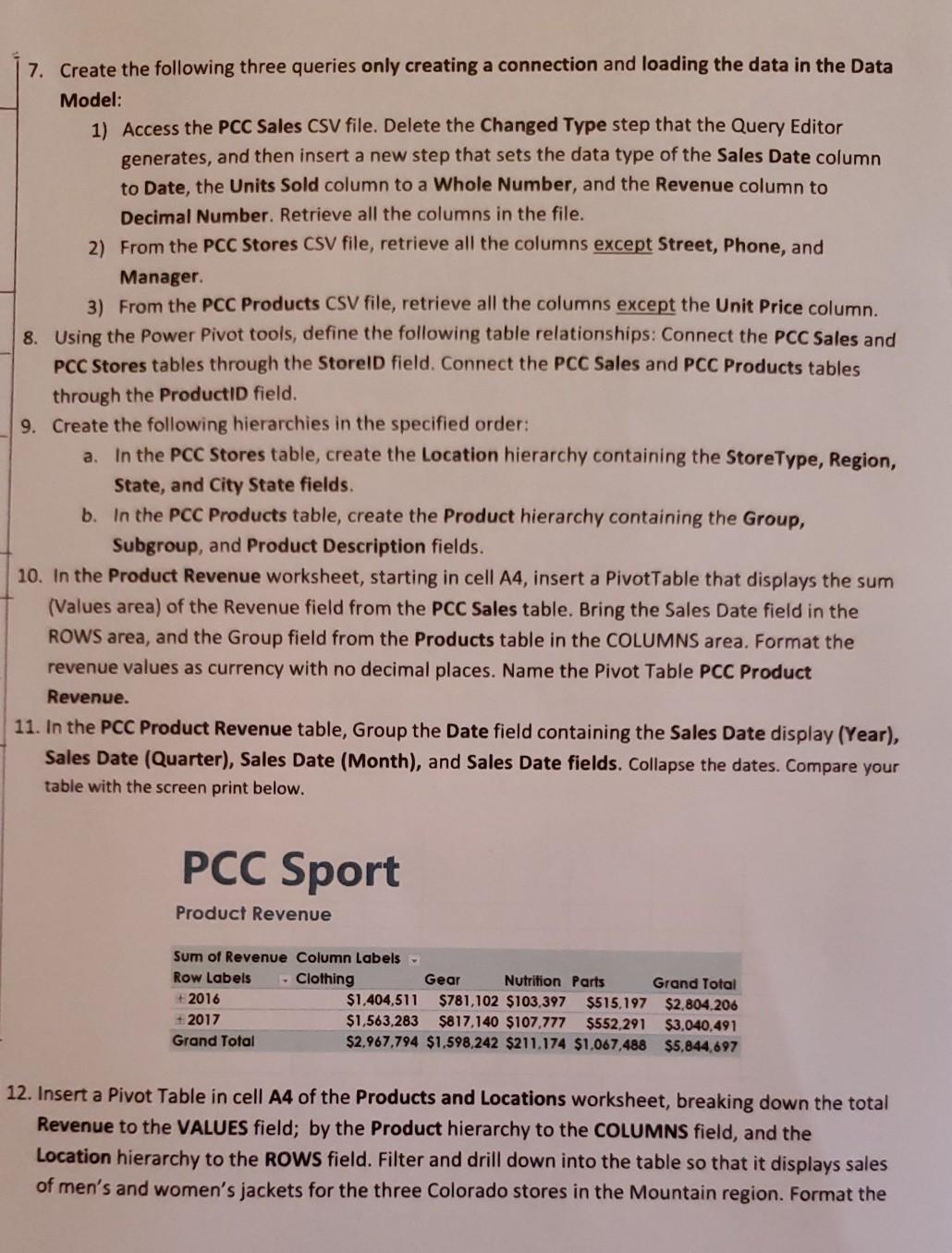
Jay Stoller is a sales analyst at PCC Sport, a chain of sporting goods stores located in the western United States. Jay is working on a sales report that will detail customer purchases of PCC Sport's line of cycling products. He has CSV files with two years of sales data. Jay wants you to compare website sales with brick-and-mortar store sales over that period. He also wants you to explore whether growing interest in women's cycling apparel is reflected in clothing sales at the company. Complete the following: 1. Open the PCC.xlsx workbook. Save the workbook as XX_PCC Sport, substituting the XX with your initials. 2. In the Documentation worksheet, enter your name and the date. 3. In the Sales Trend worksheet, use the Query Editor to connect to the PCC Sales CSV file. a. Remove all columns except the Sales Date and Revenue columns. b. Create a column named Month that stores the end of month date for each transaction. C. Group the data by the Month column, creating a new column named Monthly Revenue that displays the sum of the revenue values. d. Change the name of the query to Monthly Revenue and then load the query to an Excel table, starting in cell A4 of the Sales Trend worksheet. e. Format the monthly revenue values in the range B5:B28 as currency with no decimal places. 4. In the Sales Trend worksheet, insert a scatter chart with straight lines of the data in the range A4:B28 resized to cover the range C4:N22. Create and format the chart and add axis titles as shown in the screen print on the next page. 5. Add a linear trendline to the chart to highlight the general trend of the monthly sales and for the two-period moving average. Compare your completed chart with the screen print on the next page 7. Create the following three queries only creating a connection and loading the data in the Data Model: 1) Access the PCC Sales CSV file. Delete the Changed Type step that the Query Editor generates, and then insert a new step that sets the data type of the Sales Date column to Date, the Units Sold column to a Whole Number, and the Revenue column to Decimal Number. Retrieve all the columns in the file. 2) From the PCC Stores CSV file, retrieve all the columns except Street, Phone, and Manager. 3) From the PCC Products CSV file, retrieve all the columns except the Unit Price column. 8. Using the Power Pivot tools, define the following table relationships: Connect the PCC Sales and PCC Stores tables through the Storeld field. Connect the PCC Sales and PCC Products tables through the ProductID field. 9. Create the following hierarchies in the specified order: a. In the PCC Stores table, create the Location hierarchy containing the StoreType, Region, State, and City State fields. b. In the PCC Products table, create the Product hierarchy containing the Group, Subgroup, and Product Description fields. 10. In the Product Revenue worksheet, starting in cell A4, insert a Pivot Table that displays the sum (Values area) of the Revenue field from the PCC Sales table. Bring the Sales Date field in the ROWS area, and the Group field from the Products table in the COLUMNS area. Format the revenue values as currency with no decimal places. Name the Pivot Table PCC Product Revenue. 11. In the PCC Product Revenue table, Group the Date field containing the Sales Date display (Year), Sales Date (Quarter), Sales Date (Month), and Sales Date fields. Collapse the dates. Compare your table with the screen print below. PCC Sport Product Revenue Sum of Revenue Column Labels Row Labels - Clothing Gear Nutrition Parts Grand Total 2016 $1,404,511 $781,102 $103,397 $515,197 $2,804.206 +2017 $1,563,283 $817,140 $107,777 $552.291 $3,040,491 Grand Total $2.967,794 $1,598,242 $211.174 $1,067,488 $5,844,697 12. Insert a Pivot Table in cell A4 of the Products and Locations worksheet, breaking down the total Revenue to the VALUES field; by the Product hierarchy to the COLUMNS field, and the Location hierarchy to the ROWS field. Filter and drill down into the table so that it displays sales of men's and women's jackets for the three Colorado stores in the Mountain region. Format the 6. Based on the data in the range A4:B28, create a forecast sheet named Revenue Forecast that projects monthly sales through 12/31/2020 assuming a 12-month seasonal period and including a 95 percent confidence interval for projections. Resize the forecast chart to cover the range C2:E23. Note that the increasingly wider confidence band around the projected values indicated that the forecast is less precise farther into the future. Move the worksheet after the Sales Trend sheet. Compare your worksheet to the screen print below. Jay Stoller is a sales analyst at PCC Sport, a chain of sporting goods stores located in the western United States. Jay is working on a sales report that will detail customer purchases of PCC Sport's line of cycling products. He has CSV files with two years of sales data. Jay wants you to compare website sales with brick-and-mortar store sales over that period. He also wants you to explore whether growing interest in women's cycling apparel is reflected in clothing sales at the company. Complete the following: 1. Open the PCC.xlsx workbook. Save the workbook as XX_PCC Sport, substituting the XX with your initials. 2. In the Documentation worksheet, enter your name and the date. 3. In the Sales Trend worksheet, use the Query Editor to connect to the PCC Sales CSV file. a. Remove all columns except the Sales Date and Revenue columns. b. Create a column named Month that stores the end of month date for each transaction. C. Group the data by the Month column, creating a new column named Monthly Revenue that displays the sum of the revenue values. d. Change the name of the query to Monthly Revenue and then load the query to an Excel table, starting in cell A4 of the Sales Trend worksheet. e. Format the monthly revenue values in the range B5:B28 as currency with no decimal places. 4. In the Sales Trend worksheet, insert a scatter chart with straight lines of the data in the range A4:B28 resized to cover the range C4:N22. Create and format the chart and add axis titles as shown in the screen print on the next page. 5. Add a linear trendline to the chart to highlight the general trend of the monthly sales and for the two-period moving average. Compare your completed chart with the screen print on the next page 7. Create the following three queries only creating a connection and loading the data in the Data Model: 1) Access the PCC Sales CSV file. Delete the Changed Type step that the Query Editor generates, and then insert a new step that sets the data type of the Sales Date column to Date, the Units Sold column to a Whole Number, and the Revenue column to Decimal Number. Retrieve all the columns in the file. 2) From the PCC Stores CSV file, retrieve all the columns except Street, Phone, and Manager. 3) From the PCC Products CSV file, retrieve all the columns except the Unit Price column. 8. Using the Power Pivot tools, define the following table relationships: Connect the PCC Sales and PCC Stores tables through the Storeld field. Connect the PCC Sales and PCC Products tables through the ProductID field. 9. Create the following hierarchies in the specified order: a. In the PCC Stores table, create the Location hierarchy containing the StoreType, Region, State, and City State fields. b. In the PCC Products table, create the Product hierarchy containing the Group, Subgroup, and Product Description fields. 10. In the Product Revenue worksheet, starting in cell A4, insert a Pivot Table that displays the sum (Values area) of the Revenue field from the PCC Sales table. Bring the Sales Date field in the ROWS area, and the Group field from the Products table in the COLUMNS area. Format the revenue values as currency with no decimal places. Name the Pivot Table PCC Product Revenue. 11. In the PCC Product Revenue table, Group the Date field containing the Sales Date display (Year), Sales Date (Quarter), Sales Date (Month), and Sales Date fields. Collapse the dates. Compare your table with the screen print below. PCC Sport Product Revenue Sum of Revenue Column Labels Row Labels - Clothing Gear Nutrition Parts Grand Total 2016 $1,404,511 $781,102 $103,397 $515,197 $2,804.206 +2017 $1,563,283 $817,140 $107,777 $552.291 $3,040,491 Grand Total $2.967,794 $1,598,242 $211.174 $1,067,488 $5,844,697 12. Insert a Pivot Table in cell A4 of the Products and Locations worksheet, breaking down the total Revenue to the VALUES field; by the Product hierarchy to the COLUMNS field, and the Location hierarchy to the ROWS field. Filter and drill down into the table so that it displays sales of men's and women's jackets for the three Colorado stores in the Mountain region. Format the 6. Based on the data in the range A4:B28, create a forecast sheet named Revenue Forecast that projects monthly sales through 12/31/2020 assuming a 12-month seasonal period and including a 95 percent confidence interval for projections. Resize the forecast chart to cover the range C2:E23. Note that the increasingly wider confidence band around the projected values indicated that the forecast is less precise farther into the future. Move the worksheet after the Sales Trend sheet. Compare your worksheet to the screen print below