

Question: .... Kindly help out 14-93 The rework time required for a machine was found to 14-95. Consider the following ANOVA table from a two-fac- depend
.... Kindly help out
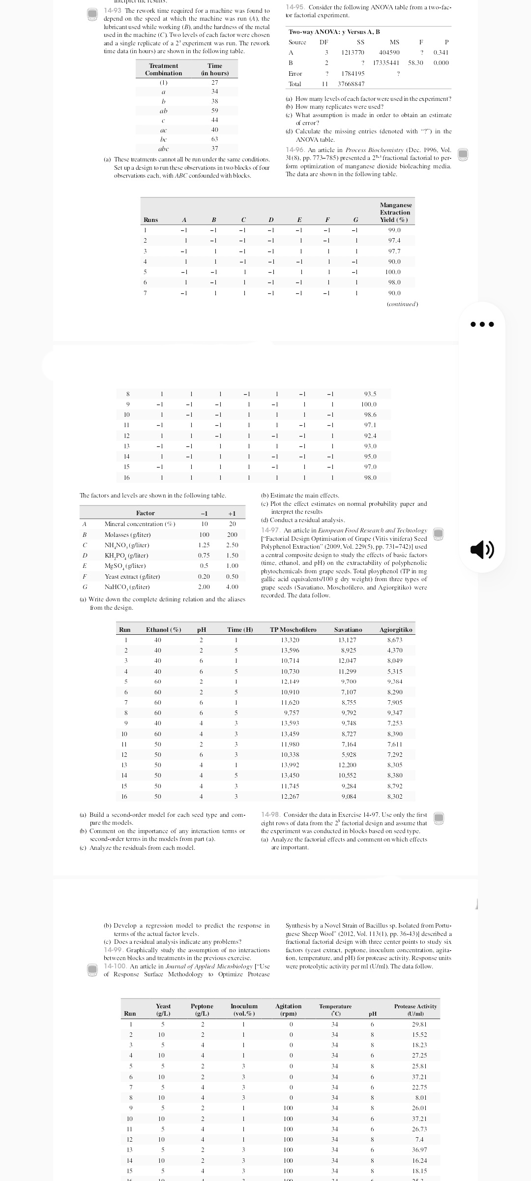
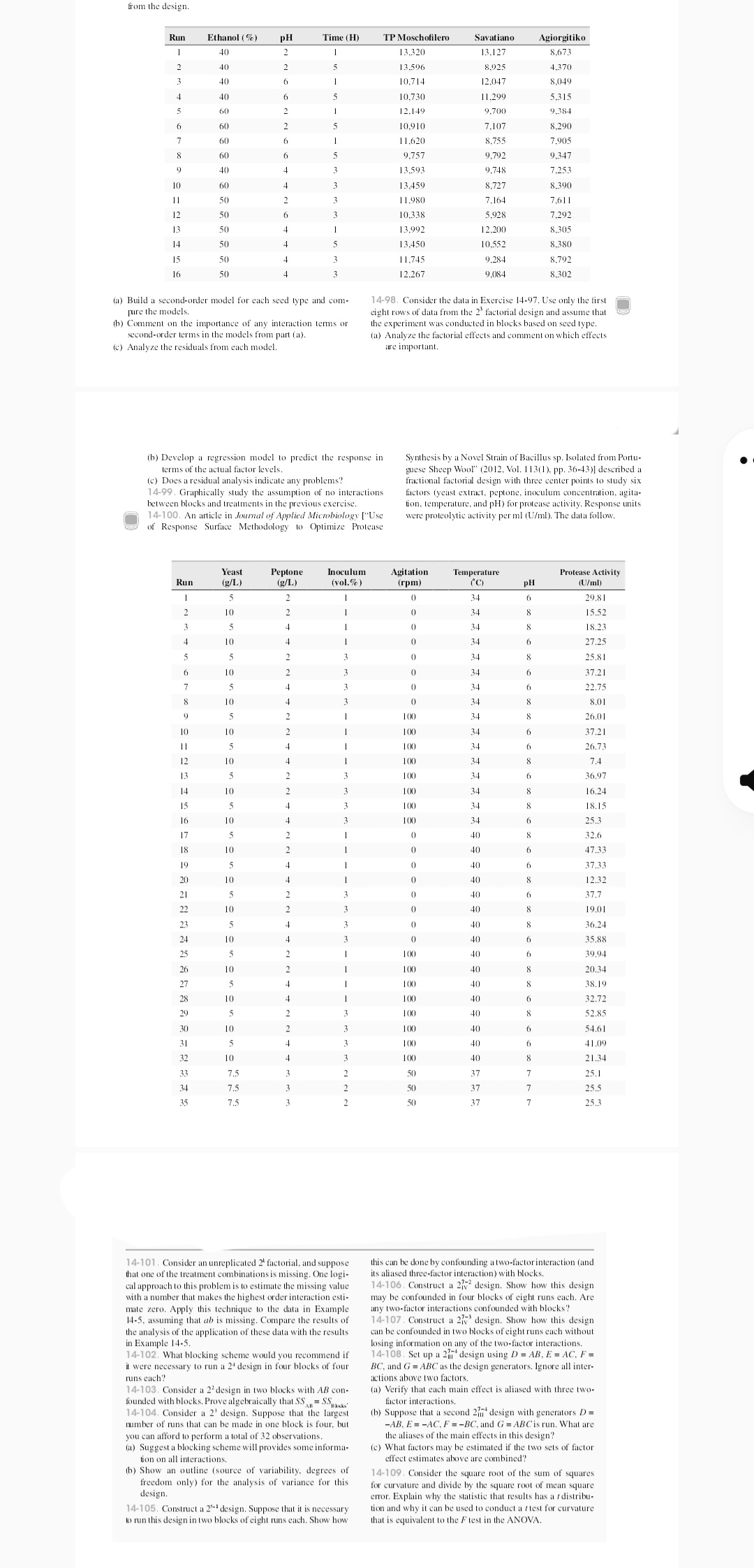
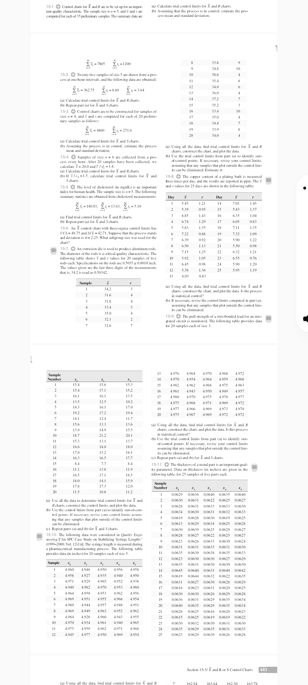
14-93 The rework time required for a machine was found to 14-95. Consider the following ANOVA table from a two-fac- depend on the speed at which the machine was run (A). the or factorial experiment. ubricant used while working (B), and the hardness of the metal used in the machine (C). Two levels of each factor were chosen Two-way ANOVA: y Versus A, B and a single replicate of a 2" experiment was run. The rework Source SS MS F P ime data (in hours) are shown in the following table. 3 1213770 404590 0.34 Treatment Time ? 17335441 58.30 0.000 Combination in hours) Fro 1784195 (1) 27 Total 37668847 34 38 (a) How many levels of each factor were used in the experiment? 50 (b) How many replicates were used? ab 44 (c) What assumption is made in order to obtain an estimate of error? ac 40 (d) Calculate the missing entries (denoted with "?") in the 63 ANOVA table. abc 37 14-96. An article in Process Biochemistry (Dec. 1996. Vol. (a) These treatments cannot all be run under the same conditions. 31 (8), pp. 773-785) presented a 2"- fractional factorial to per- Set up a design to run these observations in two blocks of four form optimization of manganese dioxide bioleaching media. observations each, with ABC confounded with blocks. The data are shown in the following table. Manganese Extraction Runs D E G Yield (%) 99.0 97.4 L - LELE 97.7 90.0 L L 00. 98.0 L - L ! 90.0 (continued) . . . 93.5 100.0 98.6 92.4 - - L. - - - 93.0 95.0 97.0 98.0 The factors and levels are shown in the following table. (b) Estimate the main effects. (c) Plot the effect estimates on normal probability paper and Factor -1 +1 interpret the results A Mineral concentration (%) 10 20 (d) Conduct a residual analysis. Molasses (gliter) 100 200 14-97. An article in European Food Research and Technology ["Factorial Design Optimisation of Grape ( Vitis vinifera) Seed NH, NO, (g/liter) 1.25 2.50 Polyphenol Extraction" (2009, Vol. 229(5), pp. 731-742)] used KH,PO, (g/liter) 0.75 1 50 a central composite design to study the effects of basic factors MgSO, (g/liter) 0.5 (time. ethanol. and pH) on the extractability of polyphenolic phytochemicals from grape seeds. Total ployphenol (TP in mg Yeast extract (gliter) 0.20 0.50 gallic acid equivalents/100 g dry weight) from three types of NaHCO, (Aliter) 2 00 4.0 grape seeds (Savatiano. Moschotilero. and Agiorgitiko) were a) Write down the complete defining relation and the aliases recorded. The data follow. from the design. Run Ethanol (7%) PH Time (H) TP Moschofilero Savatiano Agiorgitiko 40 13.320 13.127 8.673 40 IN I 13.596 8.925 4.370 10.714 12.047 8.049 40 .730 11.299 5.315 60 12,149 9.700 9.384 60 10.9 7,107 8.290 60 11.620 3.755 7.905 60 9,757 9.792 9.347 40 13.593 9.748 7.253 60 13.459 8.727 8.390 11,980 7,164 7.611 10.338 5.928 7.292 13.992 2.200 8.305 13.450 10.552 8.380 50 1 1,745 9.284 8.792 50 12.267 .084 8.302 (a) Build a second-order model for each seed type and com- 14-98. Consider the data in Exercise 14-97. Use only the first pare the models. cight rows of data from the 2' factorial design and assume that (b) Comment on the importance of any interaction terms or the experiment was conducted in blocks based on seed type second-order terms in the models from part (a). a) Analyze the factorial effects and comment on which effects (c) Analyze the residuals from each model. are important. (b) Develop a regression model to predict the response in Synthesis by a Novel Strain of Bacillus sp. Isolated from Portu- terms of the actual factor levels. guese Sheep Wool" (2012, Vol. 1 13(1), pp. 36-43)] described a (c) Does a residual analysis indicate any problems? fractional factorial design with three center points to study six 14-99. Graphically study the assumption of no interactions factors (yeast extract, peptone, inoculum concentration, agita- between blocks and treatments in the previous exercise. ion, temperature, and pH) for protease activity. Response units 14-100. An article in Journal of Applied Microbiology ["Use were proteolytic activity per ml (U/ml). The data follow. of Response Surface Methodology to Optimize Protease Yeast Peptone noculum Agitation Temperature Protease Activity Run (g/L (9/L) (vol.%) (rpm) PH (U/ml) 34 29.81 10 34 15.52 34 18.23 10 34 27.25 5 34 25.81 10 34 37.21 5 34 22.75 10 0 34 8.01 100 34 8 26.01 100 34 37.2 100 34 26.73 100 74 100 36.97 NN 16.24 w " 18.15from the design. Run Ethanol (%) PH Time (H) TP Moschofilero Savatiano Agiorgitiko 40 13.320 13.127 8.673 40 13.596 8.925 4.370 40 10.714 12.047 8.049 of 10,730 11,299 5.315 60 12.149 9.700 9.384 60 10.910 7.107 8.290 60 11.620 8,755 7.905 60 9.757 9,792 9.347 40 13.593 9,748 7.253 60 13.459 8,727 8.390 11.980 7.164 7.611 10.338 5.928 7.292 13.992 12.200 8.305 13,450 10.552 8.380 11.745 9.284 8.792 16 12.267 9.084 8.302 a) Build a second-order model for each seed type and com- 14-98. Consider the data in Exercise 14-97. Use only the first pure the models. eight rows of data from the 2' factorial design and assume that b) Comment on the importance of any interaction terms or the experiment was conducted in blocks based on seed type. second-order terms in the models from part (a). (a) Analyze the factorial effects and comment on which effects (c) Analyze the residuals from each model. are important. (b) Develop a regression model to predict the response in Synthesis by a Novel Strain of Bacillus sp. Isolated from Portu- terms of the actual factor levels. guese Sheep Wool" (2012, Vol. 1 13(1), pp. 36-43)] described a (c) Does a residual analysis indicate any problems? fractional factorial design with three center points to study six 14-99. Graphically study the assumption of no interactions factors (yeast extract, peptone, inoculum concentration, agita- between blocks and treatments in the previous exercise. tion, temperature, and pH) for protease activity. Response units 14-100. An article in Journal of Applied Microbiology ["Use were proteolytic activity per ml (U/ml). The data follow. of Response Surface Methodology to Optimize Protease Yeast Peptone Inoculum Agitation Temperature Protease Activity Run (g/L) (g/L) (vol.%) (rpm) (c) PH (U/ml) 34 29.81 10 N 34 15.52 W N 34 18.23 10 34 27.25 5 34 25.81 N N . 10 34 37.21 5 34 22.75 10 34 8.01 100 26.01 37.21 26.73 - ANNAANNA 74 36.97 16.24 18.15 25.3 32.6 47.33 37.33 2.32 37.7 19.01 688 8 8 8 8 8 8 . 9 9 9 9 - 8 8 8 8 8 8 8 36.24 35.88 39.94 20.34 38.19 32.72 52.85 54.61 41.09 21.34 25.1 25.5 25.3 14-101. Consider an unreplicated 2" factorial, and suppose this can be done by confounding a two-factor interaction (and that one of the treatment combinations is missing. One logi- its aliased three-factor interaction) with blocks. cal approach to this problem is to estimate the missing value 14-106. Construct a 2;v design. Show how this design with a number that makes the highest order interaction esti- may be confounded in four blocks of eight runs each. Are mate zero. Apply this technique to the data in Example any two-factor interactions confounded with blocks? 14-5, assuming that ab is missing. Compare the results of 14-107. Construct a 2j' design, Show how this design the analysis of the application of these data with the results can be confounded in two blocks of eight runs each without in Example 14-5. losing information on any of the two-factor interactions. 14-102. What blocking scheme would you recommend if 14-108. Set up a 2mi design using D = AB, E = AC, F= i were necessary to run a 2" design in four blocks of four BC, and G = ABC as the design generators. Ignore all inter- runs each? actions above two factors. 14-103, Consider a 2" design in two blocks with AB con- (a) Verify that each main effect is aliased with three two- founded with blocks. Prove algebraically that SS= SS, factor interactions. 14-104, Consider a 2' design. Suppose that the largest b) Suppose that a second 2hi" design with generators D = number of runs that can be made in one block is four, but -AB, E = -AC, F = -BC, and G = ABC is run. What are you can afford to perform a total of 32 observations. the aliases of the main effects in this design? (a) Suggest a blocking scheme will provides some informa- c) What factors may be estimated if the two sets of factor tion on all interactions. effect estimates above are combined? b) Show an outline (source of variability, degrees of 14-109. Consider the square root of the sum of squares freedom only) for the analysis of variance for this for curvature and divide by the square root of mean square design. error. Explain why the statistic that results has a / distribu- 14-105. Construct a 2"- design. Suppose that it is necessary tion and why it can be used to conduct a f test for curvature to run this design in two blocks of eight runs each. Show how that is equivalent to the F test in the ANOVA.15-1. + Control charts for X and R are to be set up for an impor- (a) Calculate trial control limits for X and R charts. tant quality characteristic. The sample size is n = 5, and X and r are (b) Assuming that the process is in control. estimate the pro- computed for each of 35 preliminary samples. The summary data are cess mean and standard deviation. Ex, = 7805 Er, = 1200 33.8 34.8 15-2. + Twenty-five samples of size 5 are drawn from a pro- 10 38.6 cess at one-hour intervals, and the following data are obtained: 11 354 F, = 362.75 4=8.60 12 34.0 Es, = 3.64 13 36.0 (a) Calculate trial control limits for X and Rcharts. 14 37.2 b) Repeat part (a) for X and Scharts. 15 35.2 15-3. + Control charts are to be constructed for samples of 16 33.4 size n = 4. and Y and s are computed for each of 20 prelimi- 17 35.0 nary samples as follows: 18 34.4 [.x, = 4460 Es, = 271.6 19 33.9 20 34.0 (a) Calculate trial control limits for X and Scharts. (b) Assuming the process is in control. estimate the process (a) Using all the data, find trial control limits for X and R mean and standard deviation. charts, construct the chart, and plot the data. 15-4. + Samples of size n = 6 are collected from a pro- (b) Use the trial control limits from part (a) to identify out- cess every hour. After 20 samples have been collected, we of-control points. If necessary, revise your control limits. calculate Y = 20.0 and 7 / dy = 1.4. assuming that any samples that plot outside the control lim- (a) Calculate trial control limits for X and Rcharts. its can be eliminated. Estimate of. (b) If 3 / c. = 1.5, calculate trial control limits for X and 15-8. + The copper content of a plating bath is measured Scharts. three times per day, and the results are reported in ppm. The .X 15-5. + The level of cholesterol (in my/dL) is an important and r values for 25 days are shown in the following table: index for human health. The sample size is n = 5. The following summary statistics are obtained from cholesterol measurements: Day X Day 5.4 7.01 [x, = 140.03. and / values for 20 samples of five 5.92 1.05 23 655 0.76 rods cach. Specifications on the rods are 0.5035 + 0.0010 inch. 64 0.98 24 5.90 1.20 The values given are the last three digits of the measurement; 12 5.38 1.36 25 595 that is. 34.2 is read as 0.50342. 1.19 13 6.03 083 Sample a) Using all the data. find trial control limits for X and R 34.2 charts, construct the chart, and plot the data. Is the process 31.6 in statistical control? W N 31.8. (b) If necessary, revise the control limits computed in part (a). 33.4 assuming that any samples that plot outside the control lim- its can be eliminated. 35.0 15-9. + The pull strength of a wire-bonded lead for an inte- 32.1 grated circuit is monitored. The following table provides data 32.6 for 20 samples each of size 3. Sample 4.976 4.964 4.970 4.968 4.972 Number 4.970 1954 4.964 1.959 4.968 15.6 4.982 4.962 4.968 1975 4.963 17.1 15.2 4.96 1.943 4.950 1.949 1.957 16.1 13.5 4.980 4.970 4.975 1.978 4.977 12.5 10.2 4.975 4.968 1.971 1.969 4.972 18.3 16.1 17.0 4.977 4.966 4.969 4.973 4.970 19.2 19.4 4.975 4.967 4.969 4.972 4.972 13 13.6 (a) Using all the data, find trial control limits for X and R 13.9 15.5 charts, construct the chart, and plot the data. Is this process 18.7 21.2 20.1 in statistical control? 11 15.3 13.1 13.7 (b) Use the trial control limits from part (a) to identify out- 16.6 18.0 of-control points. If necessary, revise your control limits 18.0 assuming that any samples that plot outside the control lim- 17.0 15.2 18.1 its can be eliminated. 16.3 16.5 17.7 (c) Repeat parts (a) and (b) for X and S charts. 8.4 7.7 8.4 15-11. + The thickness of a metal part is an important qual- 16 11.1 13.8 11.9 ity parameter. Data on thickness (in inches) are given in the 16.5 17.1 18.5 following table, for 25 samples of five parts each. 18 18.0 14.1 15.9 19 178 17.3 Sample 12.0 Number 115 10.8 112 0.0629 0.0636 0.0640 0.0635 0.0640 (a) Use all the data to determine trial control limits for X and 0.0630 0.0631 0.0622 0.0625 0.0627 Rcharts, construct the control limits, and plot the data. 0.0628 0.0631 0.0633 0.0633 0.0630 (b) Use the control limits from part (a) to identify out-of-con- tol points. If necessary, revise your control limits assum- 0.0634 0.0630 0.0631 0.0632 0.063. ing that any samples that plot outside of the control limits 0.0619 0.0628 0.0630 0.0619 0.0625 can be eliminated. 0.0613 0.0629 0.0634 0.0625 0.0628 (c) Repeat parts (a) and (b) for X and Scharts. 0.0630 0.0639 0.0625 0.0629 0.0627 15-10. The following data were considered in Quality Engi- 0.0628 0.0627 0.0622 0.0625 0.0627 neering ["An SPC Case Study on Stabilizing Syringe Lengths" (1999-2000. Vol. 12(1))]. The syringe length is measured during 0.0623 0.0626 0.0633 0.0630 0.0624 a pharmaceutical manufacturing process. The following table 0.0631 0.0631 0.0633 0.0631 0.0630 provides data (in inches) for 20 samples each of size 5. 0.0635 0.0630 0.0638 0.0635 0.0633 12 0.0623 0.0630 0.0630 0.0627 0.0629 Sample 0.0635 0.0631 0.0630 0.0630 0.0630 4.960 4.946 4.950 4.956 4.958 0.0645 0.0640 0.0631 0.0640 0.0642 4.958 4.927 4.935 4.940 4.950 0.0619 0.0644 0.0632 0.0622 0.0635 1.971 4.929 4.965 1.952 4.938 0.0631 0.0627 0.0630 0.0628 0.0629 1940 4.982 4.970 4.953 4.960 0.0616 0.0623 0.0631 0.0620 0.062: 1.964 4.950 4.953 1.962 4.956 0.0630 0.0630 0.0626 0.0629 0.0628 4.969 1.951 4.955 4.966 4.954 0.0636 0.0631 0.0629 0.0635 0.0634 4.960 4.944 4.957 4.948 1.951 0.0640 0.0635 0.0629 0.0635 0.0634 4.969 4.949 4.963 4.952 1.962 0.0628 0.0625 0.0616 0.0620 0.062. 1.984 4.928 4,960 194 4.955 0.0615 0.0625 0.0619 0.0619 0.0622 10 1970 4.934 4.961 194 4965 0.0630 0.0632 0.0630 0.0631 0.0630 1975 4.959 4.962 4971 4.968 0.0635 0.0629 0.0635 0.0631 0.0633 12 4.945 4.977 4.950 4,969 4.954 0.0623 0.0629 0.0630 0.0626 0.0628 Section 15-3/ X and R or S Control Charts 683
Step by Step Solution
There are 3 Steps involved in it

Get step-by-step solutions from verified subject matter experts