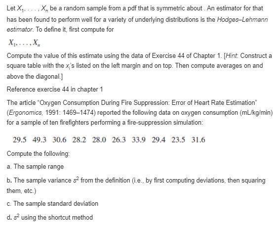
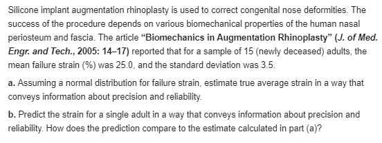
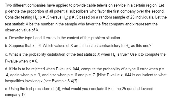
kindly solve the question

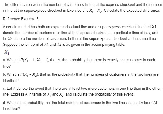
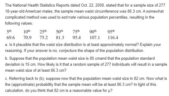
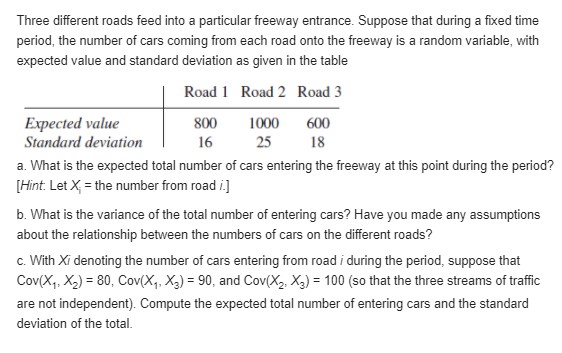
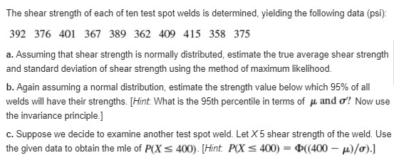
The difference between the number of customers in line at the express checkout and the number in line at the superexpress checkout in Exercise 3 is X, - X2 Calculate the expected difference. Reference Exercise 3 A certain market has both an express checkout line and a superexpress checkout line. Let X1 denote the number of customers in line at the express checkout at a particular time of day, and let X2 denote the number of customers in line at the superexpress checkout at the same time. Suppose the joint pmf of X1 and X2 is as given in the accompanying table. X a. What is P(X, = 1, X, = 1), that is, the probability that there is exactly one customer in each line? b. What is P(X, = X,), that is, the probability that the numbers of customers in the two lines are identical? c. Let A denote the event that there are at least two more customers in one line than in the other line. Express A in terms of X, and X2, and calculate the probability of this event. d. What is the probability that the total number of customers in the two lines is exactly four? At least four?The National Health Statistics Reports dated Oct. 22, 2003, stated that for a sample size of 2?? 13yearold Ameri can males, the sample mean waist circumference was 85.3 cm. A. somewhat complicated method was used to estimate various population percentiles, resulting in the following values: 5lil It)" 25" 50:Ill T5\" 90" 95" 69.6 'l'iflslall 735.2 31.3 95.4 lll 1 16.4 a. Is it plausible that the waist size distribution is at least approximately normal?\" Explain your reasoning. lfyour answer is no, conjecture the shape of the population distribution. b. Suppose that the population mean waist size is 85 crnand that the population standard deviation is 15 cm. How likely is it that a random sample of 2?? individuals will result in a sample mean waist size of at least 86.3 cm? c. Referring back to {b}, suppose now that the population mean waist size in 82 cm. Now what is the {approximate} probability that the sample mean will be at least 85.3 cm? In light of this calculation, do you think that 82 cm is a reasonable value for p'? Three different roads feed into a particular freeway entrance. Suppose that during a fixed time period, the number of cars coming from each road onto the freeway is a random variable, with expected value and standard deviation as given in the table Road 1 Road 2 Road 3 Expected value 800 1000 600 Standard deviation 16 25 18 a. What is the expected total number of cars entering the freeway at this point during the period? [Hint: Let X = the number from road .] b. What is the variance of the total number of entering cars? Have you made any assumptions about the relationship between the numbers of cars on the different roads? c. With Xi denoting the number of cars entering from road / during the period, suppose that Cov(X,. X2) = 80, Cov(X,, X;) = 90, and Cov(X2, X,) = 100 (so that the three streams of traffic are not independent). Compute the expected total number of entering cars and the standard deviation of the total.The shear strength of each of ten test spot welds is determined, yielding the following data (psi): 392 376 401 367 389 362 409 415 358 375 a. Assuming that shear strength is normally distributed, estimate the true average shear strength and standard deviation of shear strength using the method of maximum likelihood. b. Again assuming a normal distribution, estimate the strength value below which 95% of all welds will have their strengths. [Hint: What is the 95th percentile in terms of / and o'? Now use the invariance principle.] c. Suppose we decide to examine another test spot weld. Let X 5 shear strength of the weld. Use the given data to obtain the mle of P(X $ 400). [Hint. P(X = 400) = ((400 - p)/o).]Let Xy, .. .. X be a random sample from a pdf that is symmetric about . An estimator for that has been found to perform well for a variety of underlying distributions is the Hodges-Lehmann estimator. To define it, first compute for X1. . . . . X Compute the value of this estimate using the data of Exercise 44 of Chapter 1. [Hint. Construct a square table with the x's listed on the left margin and on top. Then compute averages on and above the diagonal.] Reference exercise 44 in chapter 1 The article "Oxygen Consumption During Fire Suppression: Error of Heart Rate Estimation" (Ergonomics, 1991: 1469-1474) reported the following data on oxygen consumption (mL/kg/min) for a sample of ten firefighters performing a fire-suppression simulation: 29.5 49.3 30.6 28.2 28.0 26.3 33.9 29.4 23.5 31.6 Compute the following: a. The sample range b. The sample variance s from the definition (i.e., by first computing deviations, then squaring them, etc.) c. The sample standard deviation d. s' using the shortcut methodSilicone implant augmentation rhinoplasty is used to correct congenital nose deformities. The success of the procedure depends on various biomechanical properties of the human nasal periosteum and fascia. The article "Biomechanics in Augmentation Rhinoplasty" (J. of Med. Engr. and Tech., 2005: 14-17) reported that for a sample of 15 (newly deceased) adults, the mean failure strain (%) was 25.0, and the standard deviation was 3.5. a. Assuming a normal distribution for failure strain, estimate true average strain in a way that conveys information about precision and reliability. b. Predict the strain for a single adult in a way that conveys information about precision and reliability. How does the prediction compare to the estimate calculated in part (a)?Two different companies have applied to provide cable television service in a certain region. Let p denote the proportion of all potential subscribers who favor the first company over the second. Consider testing H.: p = .5 versus H,: p # .5 based on a random sample of 25 individuals. Let the test statistic X be the number in the sample who favor the first company and x represent the observed value of X. a. Describe type I and II errors in the context of this problem situation. b. Suppose that x = 6. Which values of X are at least as contradictory to H. as this one? c. What is the probability distribution of the test statistic X when H, is true? Use it to compute the P-value when x = 6. d. If Ho is to be rejected when P-values .044, compute the probability of a type II error when p = 4, again when p = .3, and also when p = .6 and p = .7. [Hint: P-value > .044 is equivalent to what inequalities involving x (see Example 8.4)?] e. Using the test procedure of (d), what would you conclude if 6 of the 25 queried favored company 1