Laurman, Inc. is considering a new project and has provided the details of the project. The Controller has asked you to compute various capital budgeting methods to help aid in the decision to pursue the investment. Use the information included in the Excel Simulation and the Excel functions described below to complete the task.

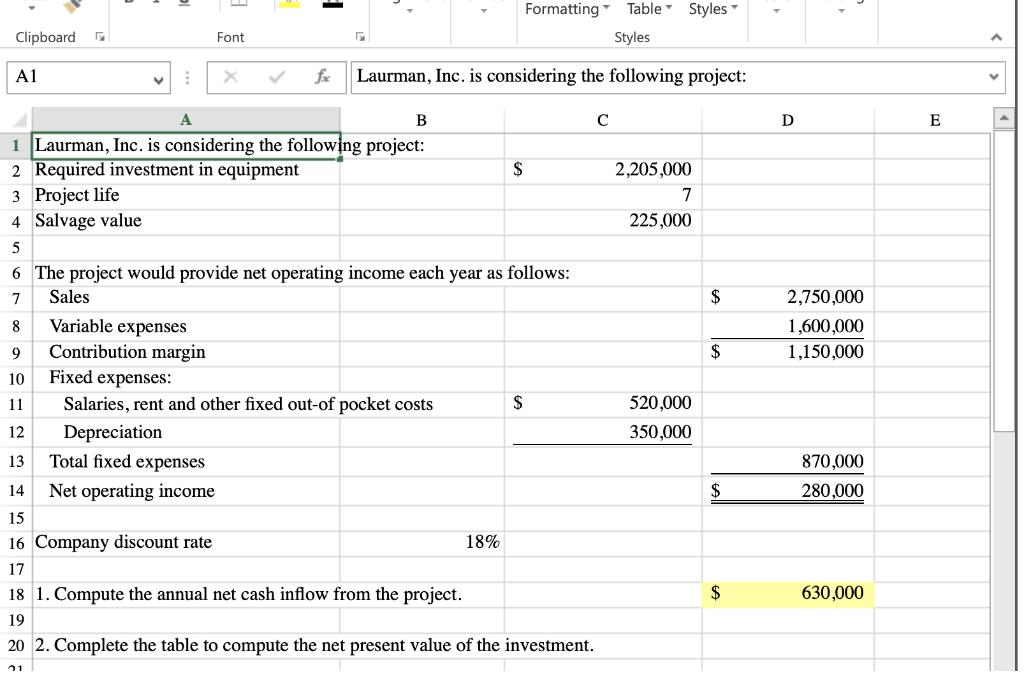
Cell Reference: Allows you to refer to data from another cell in the worksheet. From the Excel Simulation below, if in a blank cell, “=C4” was entered, the formula would output the result from cell C4, or 225,000,000 in this example.

Basic Math functions: Allows you to use the basic math symbols to perform mathematical functions. You can use the following keys: + (plus sign to add), - (minus sign to subtract), * (asterisk sign to multiply), and / (forward slash to divide). From the Excel Simulation below, if in a blank cell “=D13+D14” was entered, the formula would add the values from those cells and output the result, or 1,150,000 in this example. If using the other math symbols the result would output an appropriate answer for its function.

SUM function: Allows you to refer to multiple cells and adds all the values. You can add individual cell references or ranges to utilize this function. From the Excel Simulation below, if in a blank cell “=SUM(D7,D8,D9)” was entered, the formula would output the result of adding those three separate cells, or 5,500,000 in this example. Similarly, if in a blank cell “=SUM(D7:D9)” was entered, the formula would output the same result of adding those cells, except they are expressed as a range in the formula, and the result would be 5,500,000 in this example.

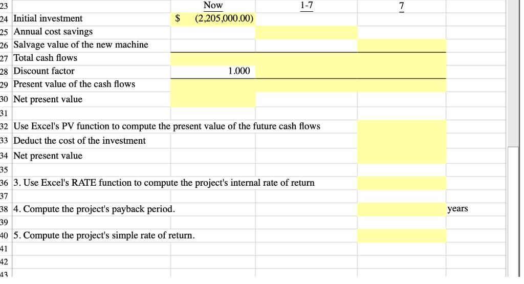
RATE function: Allows you to return the interest rate per period. The syntax of the RATE function is “=RATE(nper,pmt,pv,[fv],[type],[guess])” and results in the percentage interest rate value for the related inputs. The nper argument is the total number of payment periods. The pmt argument is the payment made each period that does not change over the life of the investment and this argument must be included if the [fv] argument is not included. The pv argument is the present value, or the total amount that series of future payments is worth now. The [fv] argument is the future value, or the cash basis to attain after the last payment is made and this argument must be included if the pmt argument is omitted. The [type] argument is a logical value of 0 or 1, which indicates when the payments are due where 1 is the payment at the beginning of the period and 0, is the payment at the end of the period. Both the [fv] and [type] values are optional arguments to have the formula work, which is why they are surrounded by brackets in the syntax, however, these values would not be entered with brackets in the actual function. The [guess] argument is also optional and is your guess for what the rate will be, however, if omitted the system assumes a guess of 10 percent.  For the purposes of this Excel Simulation, please include both the [pmt] and [fv] arguments, but leave out the [type] and [guess] arguments from the function. Also, the pv argument should be entered as negative value.

PV Function: Allows you to perform the mathematical present value calculation of a value. The syntax of the PV function is “=PV(rate,nper,pmt,[fv],[type])” and results in the total amount that a series of future payments is worth now also known as the present value. The rate argument is the interest rate per period. The nper argument is the total number of payment periods. The pmt argument is the payment made each period that does not change over the life of the investment and this argument must be included if the [fv] argument is not included. The [fv] argument is the future value, or the cash basis to attain after the last payment is made and this argument must be included if the pmt argument is omitted. The [type] argument is a logical value of 0 or 1, which indicates when the payments are due where 1 is the payment at the beginning of the period and 0, is the payment at the end of the period. Both the [fv] and [type] values are optional arguments to have the formula work, which is why they are surrounded by brackets in the syntax, however, these values would not be entered with brackets in the actual function.  For the purposes of this Excel Simulation, please include both the [pmt] and [fv] arguments, but leave out the [type] argument from the function. Also, the entire PV function should have a minus sign included before the formula so the calculation will result in a positive value (i.e. “=-PV(A1,A2,A3,A4).”

  
 

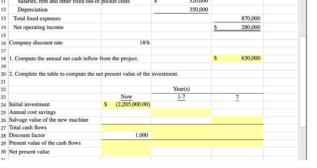
Formatting Table Styles Clipboard Font Styles A1 Laurman, Inc. is considering the following project: B C D E 1 Laurman, Inc. is considering the following project: 2 Required investment in equipment 3 Project life 4 Salvage value 2$ 2,205,000 7 225,000 5 6 The project would provide net operating income each year as follows: Sales $ 2,750,000 Variable expenses Contribution margin Fixed expenses: 8 1,600,000 9 $ 1,150,000 10 11 Salaries, rent and other fixed out-of pocket costs $ 520,000 Depreciation Total fixed expenses 12 350,000 13 870,000 14 Net operating income $ 280,000 15 16 Company discount rate 18% 17 18 1. Compute the annual net cash inflow from the project. 2$ 630,000 19 20 2. Complete the table to compute the net present value of the investment.