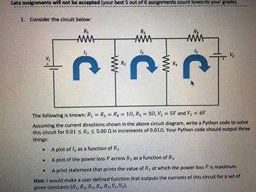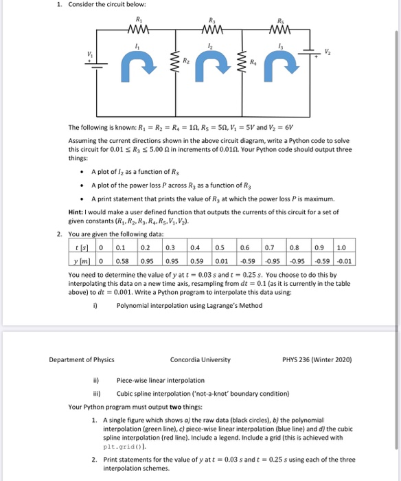
Lite assignments will not be accepted your best out of ag ent count towards your 1 Consider the circuit below The following is known: R R -R-10, R, S,V, SV and V, - 6V Assuming the current directions shown in the above circuit diagram, write a Python code to solve this circuit for 0.01 SR, S5.00 nin increments of 0.010. Your Python code should output three things: A plot ofl, as a function of R A plot of the power loss Pacross R, as a function of A print statement that prints the value of R, at which the power loss Pls maximum Hint: I would make a user defined function that outputs the currents of this c ut for a set of Even constants (R.RRR.NVV.. 1. Consider the circuit below: The following is known: R = R2 = R = 19, Rs = 50, V = 5V and V2 = 6V Assuming the current directions shown in the above circuit diagram, write a Python code to solve this circuit for 0.01 S R S 5.00 in increments of 0.019. Your Python code should output three things: A plot of 12 as a function of R3 A plot of the power loss Pacross Rg as a function of R3 A print statement that prints the value of R, at which the power loss P is maximum. Hint: I would make a user defined function that outputs the currents of this circuit for a set of given constants (R.R.R.R.R.V.12). You are given the following data: Les o 0.1 0.2 0.3 0.4 0.5 0.6 0.7 0.8 0.9 10 y (m) 0 0.58 0.95 0.95 0.59 0.01 -0.59 -0.95 -0.95 -0.59 -0.01 You need to determine the value of y at t = 0.03 s and t = 0.25 s. You choose to do this by interpolating this data on a new time axis, resampling from dt = 0.1 (as it is currently in the table above) to dt = 0.001. Write a Python program to interpolate this data using: 1) Polynomial interpolation using Lagrange's Method Department of Physics Concordia University PHYS 236 (Winter 2020) ii) Piece-wise linear interpolation 1) Cubic spline interpolation ('not-a-knot' boundary condition) Your Python program must output two things: 1. A single figure which shows a) the raw data (black circles), b) the polynomial interpolation (green line). c) piece-wise linear interpolation (blue line) and d) the cubic spline interpolation (red line). Include a legend. Include a grid (this is achieved with plt.grid)) 2. Print statements for the value of y at t = 0.03 s and t = 0.25 s using each of the three interpolation schemes. Lite assignments will not be accepted your best out of ag ent count towards your 1 Consider the circuit below The following is known: R R -R-10, R, S,V, SV and V, - 6V Assuming the current directions shown in the above circuit diagram, write a Python code to solve this circuit for 0.01 SR, S5.00 nin increments of 0.010. Your Python code should output three things: A plot ofl, as a function of R A plot of the power loss Pacross R, as a function of A print statement that prints the value of R, at which the power loss Pls maximum Hint: I would make a user defined function that outputs the currents of this c ut for a set of Even constants (R.RRR.NVV.. 1. Consider the circuit below: The following is known: R = R2 = R = 19, Rs = 50, V = 5V and V2 = 6V Assuming the current directions shown in the above circuit diagram, write a Python code to solve this circuit for 0.01 S R S 5.00 in increments of 0.019. Your Python code should output three things: A plot of 12 as a function of R3 A plot of the power loss Pacross Rg as a function of R3 A print statement that prints the value of R, at which the power loss P is maximum. Hint: I would make a user defined function that outputs the currents of this circuit for a set of given constants (R.R.R.R.R.V.12). You are given the following data: Les o 0.1 0.2 0.3 0.4 0.5 0.6 0.7 0.8 0.9 10 y (m) 0 0.58 0.95 0.95 0.59 0.01 -0.59 -0.95 -0.95 -0.59 -0.01 You need to determine the value of y at t = 0.03 s and t = 0.25 s. You choose to do this by interpolating this data on a new time axis, resampling from dt = 0.1 (as it is currently in the table above) to dt = 0.001. Write a Python program to interpolate this data using: 1) Polynomial interpolation using Lagrange's Method Department of Physics Concordia University PHYS 236 (Winter 2020) ii) Piece-wise linear interpolation 1) Cubic spline interpolation ('not-a-knot' boundary condition) Your Python program must output two things: 1. A single figure which shows a) the raw data (black circles), b) the polynomial interpolation (green line). c) piece-wise linear interpolation (blue line) and d) the cubic spline interpolation (red line). Include a legend. Include a grid (this is achieved with plt.grid)) 2. Print statements for the value of y at t = 0.03 s and t = 0.25 s using each of the three interpolation schemes


