Answered step by step
Verified Expert Solution
Question
1 Approved Answer
make the SciLab programming language to solve the direct synthesis problem Use the DS design method to calculate PID controller settings for the process: G=(10s+1)(5s+1)2es
make the SciLab programming language to solve the direct synthesis problem 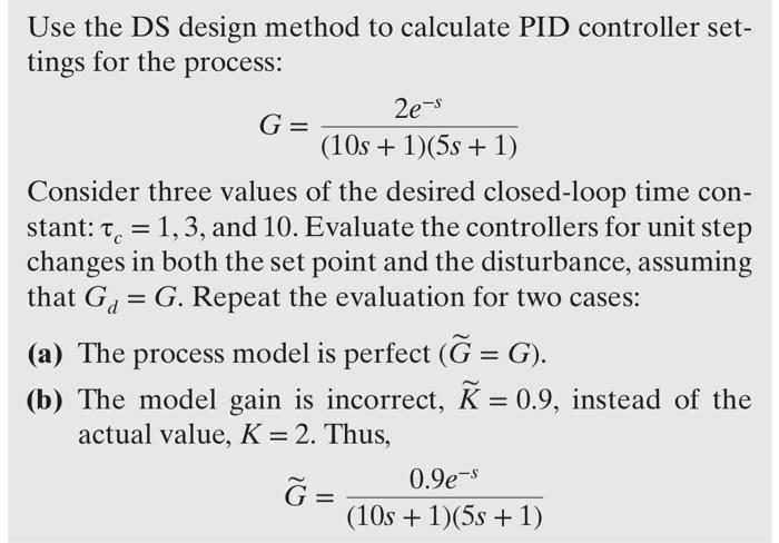
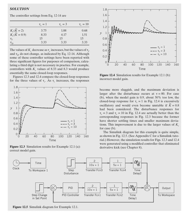
Use the DS design method to calculate PID controller settings for the process: G=(10s+1)(5s+1)2es Consider three values of the desired closed-loop time constant: c=1,3, and 10 . Evaluate the controllers for unit step changes in both the set point and the disturbance, assuming that Gd=G. Repeat the evaluation for two cases: (a) The process model is perfect (G=G). (b) The model gain is incorrect, K=0.9, instead of the actual value, K=2. Thus, G=(10s+1)(5s+1)0.9es SOLUTION The controller settings from Eq. 12-14 are The values of K decrease as increases, but the values of f and tD do not change, as indicated by Eq. 12-14. Although some of these controller settings have been reported with three significant figures for purposes of comparison, calculating a third digit is not necessary in practice. For example, controllers with Kc values of 8.33 and 8.3 would produce essentially the same closed-loop responses. Figures 12.3 and 12.4 compare the closed-loop responses for the three values of q. As c increases, the responses Figure 12.3 Simulation results for Example 12.1 (a): correct model gain. Figure 12.4 Simulation results for Example 12.1 (b): incorrect model gain. become more sluggish, and the maximum deviation is larger after the disturbance occurs at =80. For case (b). when the model gain is 0.9 , about 50% too low, the closed-loop response for tf=1 in Fig 12.4 is excessively oscillatory and would even become unstable if K=0.8 had been considered. The disturbance responses for c=3 and c=10 in Fig. 12.4 are actually better than the corresponding responses in Fig. 12.3 because the former have shorter settling times and smaller maximum deviations. This improvement is due to the larger values of K. for case (b). The Simulink diagram for this example is quite simple, as shown in Fig. 12.5. (See Appendix C for a Simulink tutorial.) However, the simulation results for Figs, 12.3 and 12.4 were generated using a modified controller that eliminated derivative kick (see Chapter 8 ). Figure 12.5 Simulink diagram for Example 12.1 

Step by Step Solution
There are 3 Steps involved in it
Step: 1

Get Instant Access to Expert-Tailored Solutions
See step-by-step solutions with expert insights and AI powered tools for academic success
Step: 2

Step: 3

Ace Your Homework with AI
Get the answers you need in no time with our AI-driven, step-by-step assistance
Get Started


