MANEGERIAL ECONOMICS

Reference:

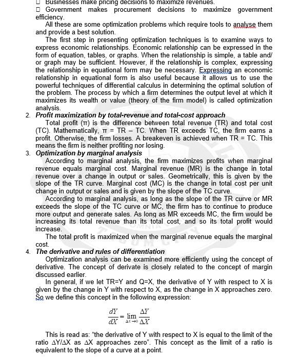
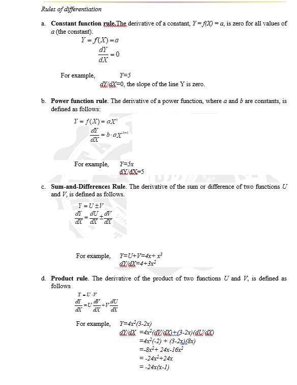
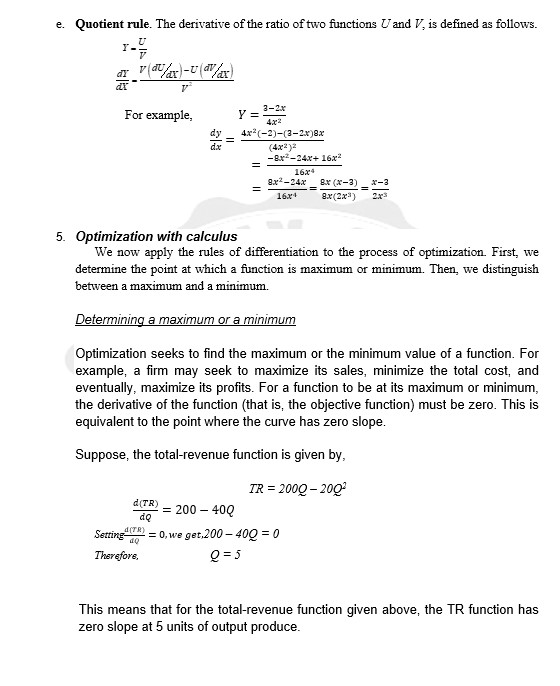
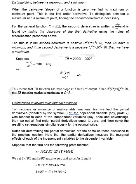
1. Optimization: Methods for maximizing or minimizing an objective function. The market is filled with optimization problems. Some of the real-world problems of optimization are as follows: Consumers make buying decisions to maximize utility (or satisfaction). Consumers make labor decisions to maximize utility (in terms of earnings) Businesses make capital investment decisions to minimize costs.Businesses make pricing decisions to maximize revenues. _ Government makes procurement decisions to maximize government efficiency. All these are some optimization problems which require tools to analyse them and provide a best solution. The first step in presenting optimization techniques is to examine ways to express economic relationships. Economic relationship can be expressed in the form of equation, tables, or graphs. When the relationship is simple, a table and/ or graph may be sufficient. However, if the relationship is complex, expressing the relationship in equational form may be necessary. Expressing an economic relationship in equational form is also useful because it allows us to use the powerful techniques of differential calculus in determining the optimal solution of the problem. The process by which a firm determines the output level at which it maximizes its wealth or value (theory of the firm model) is called optimization analysis. 2. Profit maximization by total-revenue and total-cost approach Total profit (wr) is the difference between total revenue (TR) and total cost (TC). Mathematically, T = TR - TC. When TR exceeds TC, the firm earns a profit. Otherwise, the firm losses. A breakeven is achieved when TR = TC. This means the firm is neither profiting nor losing. 3. Optimization by marginal analysis According to marginal analysis, the firm maximizes profits when marginal revenue equals marginal cost. Marginal revenue (MR) is the change in total revenue over a change in output or sales. Geometrically, this is given by the slope of the TR curve. Marginal cost (MC) is the change in total cost per unit change in output or sales and is given by the slope of the TC curve. According to marginal analysis, as long as the slope of the TR curve or MR exceeds the slope of the TC curve or MC, the firm has to continue to produce more output and generate sales. As long as MR exceeds MC, the firm would be increasing its total revenue than its total cost, and so its total profit would increase. The total profit is maximized when the marginal revenue equals the marginal cost. 4. The derivative and rules of differentiation Optimization analysis can be examined more efficiently using the concept of derivative. The concept of derivate is closely related to the concept of margin discussed earlier. In general, if we let TR=Y and Q=X, the derivative of Y with respect to X is given by the change in Y with respect to X, as the change in X approaches zero. So we define this concept in the following expression: dy AY LX lim AY40 AX This is read as: "the derivative of Y with respect to X is equal to the limit of the ratio AY/AX as AX approaches zero". This concept as the limit of a ratio is equivalent to the slope of a curve at a point.Rules of differentiation a. Constant function rule The derivative of a constant, Y=(X) = a, is zero for all values of a (the constant). Y = /(X) =a dy dx For example, Y=5 W/X=0, the slope of the line Y is zero. b. Power function rule. The derivative of a power function, where a and b are constants, is defined as follows: Y = /(n)=ax dy For example, Y=5x dy/dx=5 c. Sum-and-Differences Rule. The derivative of the sum or difference of two functions U and V', is defined as follows. di _ du _ dy For example, Y=D+V=4x+ x Max=4+3x- d. Product rule. The derivative of the product of two functions U and , is defined as follows Y - U.V dy LX For example, Y=4x-(3-2x) didx =4x(dVan+ (3-2x)(du//4x) =4x-(-2) + (3-2x)(8x) =-8x-+ 24x-16x- = -24x3+24x = -24x(x-])e. Quotient rule. The derivative of the ratio of two functions U and , is defined as follows. 3-2x For example, V=- 4x2 dy 4x3 (-2)-(3-2x)8x 4x2)2 -8x--24x+ 16x2 = 1624 9x2-24x BY (X-3) X-3 1624 9x(2x3) 2x3 5. Optimization with calculus We now apply the rules of differentiation to the process of optimization. First, we determine the point at which a function is maximum or minimum. Then, we distinguish between a maximum and a minimum. Determining a maximum or a minimum Optimization seeks to find the maximum or the minimum value of a function. For example, a firm may seek to maximize its sales, minimize the total cost, and eventually, maximize its profits. For a function to be at its maximum or minimum, the derivative of the function (that is, the objective function) must be zero. This is equivalent to the point where the curve has zero slope. Suppose, the total-revenue function is given by, TR = 200Q - 200 d(TR) = 200 -40Q do Setting aq "(TR) = 0, we get.200 - 400 = 0 Therefore, 0 =5 This means that for the total-revenue function given above, the TR function has zero slope at 5 units of output produce.Distinguishing between a maximum and a minimum When the derivative (slope) of a function is zero, we find its maximum or minimum point. This is the first order derivative. To distinguish between a maximum and a minimum point, finding the second derivative is necessary. For the general function Y = f(x), the second derivative is written as = Theand is found by taking the derivative of the first derivative using the rules of differentiation presented above. The rule is if the second derivative is positive (o Y/dX > 0), then we have a minimum, and if the second derivative is a negative (d'Y/d)