MATLAB code:

L=1; H=2; %%% BC is u(0,y)=g(y)=100 [X,Y]=meshgrid(0:.01:L,0:.01:H); for j=1:100 if j==1 Z=200*((-1)^j-1).*sinh(j*pi*(X-L)./H).*sin(j*pi*Y./H)./j./pi./sinh(j*pi*(L)./H); else ZZ=Z+200*((-1)^j-1).*sinh(j*pi*(X-L)./H).*sin(j*pi*Y./H)./j./pi./sinh(j*pi*(L)./H); Z=ZZ; end end %%% BC is u(0,y)=g(y)=100 sin(pi*y/H); Z1=-100.*sinh(pi*(X-L)./H).*sin(pi*Y./H)/sinh(pi*(L)./H);

figure (1) subplot(131),plot(Y(:,1),ZZ(:,1)) hold on plot(Y(:,1),Z1(:,1),'r') xlabel('y') ylabel('u(0,y)') legend('ZZ','Z1') title('Boundary conditions') subplot(132) [Czz,hzz]=contourf(X,Y,ZZ); colormap('cool') colorbar clabel(Czz,hzz) xlabel('x') ylabel('y')

title('u(0,y)=g(y)=100, Gibbs') %%% BC is u(0,y)=g(y)=100 sin(pi*y/H);

subplot(133)

[Cz1,hz1]=contourf(X,Y,Z1); colormap('cool') colorbar clabel(Cz1,hz1) title('u(0,y)=g(y)=100 sin(pi*y/H)') xlabel('x') ylabel('y')

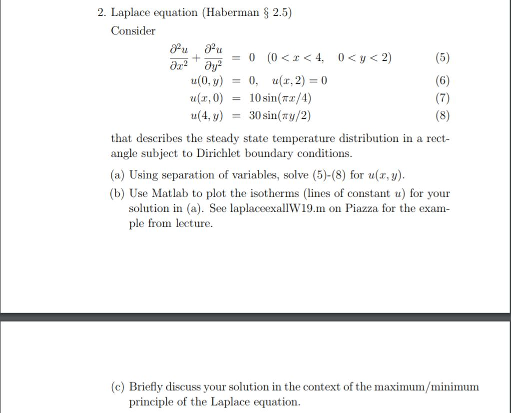
2, Laplace equation (Haberman 2.5) Consider 0, u(x, 2) 10sin(nx/4) 30 sin(ny/2) that describes the steady state temperature distribution in a rect- u(0, y- a(x,0) a(49) 0 = = angle subject to Dirichlet boundary conditions (a) Using separation of variables, solve (5)-(8) for u(x, y). (b) Use Matlab to plot the isotherms (lines of constant u) for your solution in (a). See laplaceexallW19.m on Piazza for the exam- ple from lecture (c) Briefly discuss your solution in the context of the maximum/minimum principle of the Laplace equation. 2, Laplace equation (Haberman 2.5) Consider 0, u(x, 2) 10sin(nx/4) 30 sin(ny/2) that describes the steady state temperature distribution in a rect- u(0, y- a(x,0) a(49) 0 = = angle subject to Dirichlet boundary conditions (a) Using separation of variables, solve (5)-(8) for u(x, y). (b) Use Matlab to plot the isotherms (lines of constant u) for your solution in (a). See laplaceexallW19.m on Piazza for the exam- ple from lecture (c) Briefly discuss your solution in the context of the maximum/minimum principle of the Laplace equation