MATLAB code plz

please use MATLAB for the coding

Thank you so much!

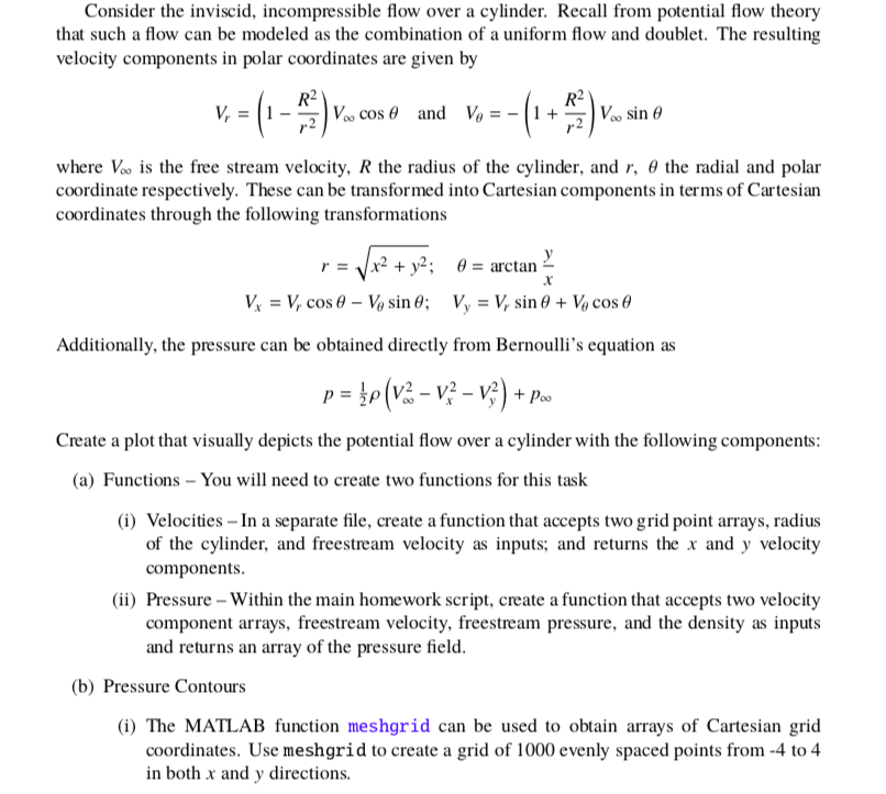
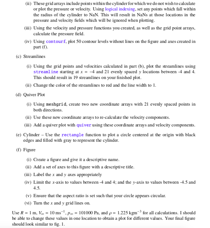
Consider the inviscid, incompressible flow over a cylinder. Recall from potential flow theory that such a flow can be modeled as the combination of a uniform flow and doublet. The resulting velocity components in polar coordinates are given by V = (1 - ) . cos 6 and Vo == (1+) V., sin where is the free stream velocity, R the radius of the cylinder, and r, the radial and polar coordinate respectively. These can be transformed into Cartesian components in terms of Cartesian coordinates through the following transformations r = V x2 + y2; 6 = arctan, Vx = V, cos 6 - V sin ; V = V, sin 0 + Ve cose Additionally, the pressure can be obtained directly from Bernoulli's equation as p = {p(V2 - V? V?) + Po Create a plot that visually depicts the potential flow over a cylinder with the following components: (a) Functions - You will need to create two functions for this task (i) Velocities - In a separate file, create a function that accepts two grid point arrays, radius of the cylinder, and freestream velocity as inputs, and returns the x and y velocity components. (ii) Pressure - Within the main homework script, create a function that accepts two velocity component arrays, freestream velocity, freestream pressure, and the density as inputs and returns an array of the pressure field. (b) Pressure Contours (i) The MATLAB function meshgrid can be used to obtain arrays of Cartesian grid coordinates. Use meshgrid to create a grid of 1000 evenly spaced points from -4 to 4 in both x and y directions. (ii) These grid arrays include points within the cylinder for which we do not wish to calculate or plot the pressure or velocity. Using logical indexing, set any points which fall within the radius of the cylinder to NaN. This will result in NaNs at those locations in the pressure and velocity fields which will be ignored when plotting. (iii) Using the velocity and pressure functions you created, as well as the grid point arrays, calculate the pressure field. (iv) Using contourf, plot 50 contour levels without lines on the figure and axes created in part (f). (c) Streamlines (i) Using the grid points and velocities calculated in part (b), plot the streamlines using streamline starting at x = 4 and 21 evenly spaced y locations between 4 and 4. This should result in 19 streamlines on your finished plot. (ii) Change the color of the streamlines to red and the line width to 1. (d) Quiver Plot (i) Using meshgrid, create two new coordinate arrays with 21 evenly spaced points in both directions. (ii) Use these new coordinate arrays to re-calculate the velocity components. (iii) Add a quiver plot with quiver using these coordinate arrays and velocity components. (e) Cylinder - Use the rectangle function to plot a circle centered at the origin with black edges and filled with gray to represent the cylinder. (f) Figure (i) Create a figure and give it a descriptive name. (ii) Add a set of axes to this figure with a descriptive title. (iii) Label the x and y axes appropriately (iv) Limit the x-axis to values between -4 and 4; and the y-axis to values between -4.5 and 4.5. (v) Ensure that the aspect ratio is set such that your circle appears circular. (vi) Turn the x and y grid lines on. Use R = 1 m, V = 10 ms.Po = 101000 Pa, and p = 1.225 kgm for all calculations. I should be able to change these values in one location to obtain a plot for different values. Your final figure should look similar to fig. 1. Consider the inviscid, incompressible flow over a cylinder. Recall from potential flow theory that such a flow can be modeled as the combination of a uniform flow and doublet. The resulting velocity components in polar coordinates are given by V = (1 - ) . cos 6 and Vo == (1+) V., sin where is the free stream velocity, R the radius of the cylinder, and r, the radial and polar coordinate respectively. These can be transformed into Cartesian components in terms of Cartesian coordinates through the following transformations r = V x2 + y2; 6 = arctan, Vx = V, cos 6 - V sin ; V = V, sin 0 + Ve cose Additionally, the pressure can be obtained directly from Bernoulli's equation as p = {p(V2 - V? V?) + Po Create a plot that visually depicts the potential flow over a cylinder with the following components: (a) Functions - You will need to create two functions for this task (i) Velocities - In a separate file, create a function that accepts two grid point arrays, radius of the cylinder, and freestream velocity as inputs, and returns the x and y velocity components. (ii) Pressure - Within the main homework script, create a function that accepts two velocity component arrays, freestream velocity, freestream pressure, and the density as inputs and returns an array of the pressure field. (b) Pressure Contours (i) The MATLAB function meshgrid can be used to obtain arrays of Cartesian grid coordinates. Use meshgrid to create a grid of 1000 evenly spaced points from -4 to 4 in both x and y directions. (ii) These grid arrays include points within the cylinder for which we do not wish to calculate or plot the pressure or velocity. Using logical indexing, set any points which fall within the radius of the cylinder to NaN. This will result in NaNs at those locations in the pressure and velocity fields which will be ignored when plotting. (iii) Using the velocity and pressure functions you created, as well as the grid point arrays, calculate the pressure field. (iv) Using contourf, plot 50 contour levels without lines on the figure and axes created in part (f). (c) Streamlines (i) Using the grid points and velocities calculated in part (b), plot the streamlines using streamline starting at x = 4 and 21 evenly spaced y locations between 4 and 4. This should result in 19 streamlines on your finished plot. (ii) Change the color of the streamlines to red and the line width to 1. (d) Quiver Plot (i) Using meshgrid, create two new coordinate arrays with 21 evenly spaced points in both directions. (ii) Use these new coordinate arrays to re-calculate the velocity components. (iii) Add a quiver plot with quiver using these coordinate arrays and velocity components. (e) Cylinder - Use the rectangle function to plot a circle centered at the origin with black edges and filled with gray to represent the cylinder. (f) Figure (i) Create a figure and give it a descriptive name. (ii) Add a set of axes to this figure with a descriptive title. (iii) Label the x and y axes appropriately (iv) Limit the x-axis to values between -4 and 4; and the y-axis to values between -4.5 and 4.5. (v) Ensure that the aspect ratio is set such that your circle appears circular. (vi) Turn the x and y grid lines on. Use R = 1 m, V = 10 ms.Po = 101000 Pa, and p = 1.225 kgm for all calculations. I should be able to change these values in one location to obtain a plot for different values. Your final figure should look similar to fig. 1