MATLAB

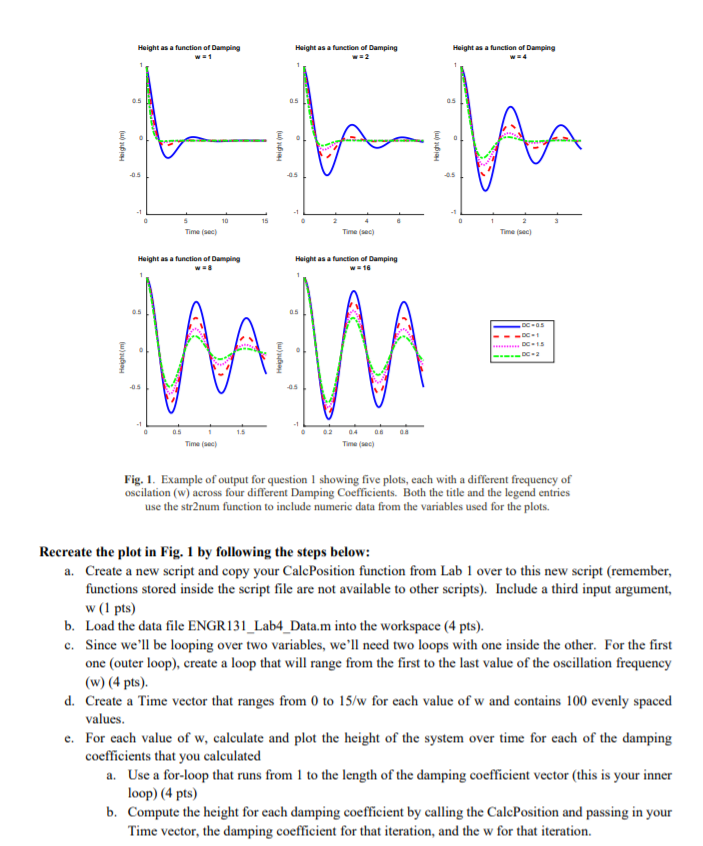
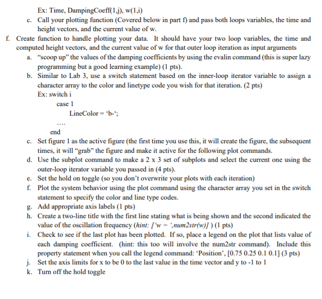
Height as a function of Damping Height as a function of Damping Height as a function of Damping -0.5 -1 o 10 15 0 3 hihih mim Time Time (e) Time Height as a function of Damping Height as a function of Damping w = 16 BC = 3 -1 1.5 04 0.6 05 1 Times) Time() Fig. 1. Example of output for question 1 showing five plots, each with a different frequency of oscilation (w) across four different Damping Coefficients. Both the title and the legend entries use the str2num function to include numeric data from the variables used for the plots. Recreate the plot in Fig. 1 by following the steps below: a. Create a new script and copy your CalcPosition function from Lab 1 over to this new script (remember, functions stored inside the script file are not available to other scripts). Include a third input argument, w (1 pts) b. Load the data file ENGR131_Lab4_Data.m into the workspace (4 pts). c. Since we'll be looping over two variables, we'll need two loops with one inside the other. For the first one (outer loop), create a loop that will range from the first to the last value of the oscillation frequency (w) (4 pts). d. Create a Time vector that ranges from 0 to 15/w for each value of w and contains 100 evenly spaced values. e. For each value of w, calculate and plot the height of the system over time for each of the damping coefficients that you calculated a. Use a for-loop that runs from 1 to the length of the damping coefficient vector (this is your inner loop) (4 pts) b. Compute the height for each damping coefficient by calling the CalcPosition and passing in your Time vector, the damping coefficient for that iteration, and the w for that iteration. Ex: Time, DampingCoeff(1.j), w(1,1) c. Call your plotting function (Covered below in part f) and pass both loops variables, the time and height vectors, and the current value of w. f. Create function to handle plotting your data. It should have your two loop variables, the time and computed height vectors, and the current value of w for that outer loop iteration as input arguments a. "scoop up" the values of the damping coefficients by using the evalin command (this is super lazy programming but a good learning example) (1 pts). b. Similar to Lab 3, use a switch statement based on the inner-loop iterator variable to assign a character array to the color and linetype code you wish for that iteration. (2 pts) Ex: switch i case 1 Line Color = 'b-"; end c. Set figure l as the active figure (the first time you use this, it will create the figure, the subsequent times, it will grab" the figure and make it active for the following plot commands. d. Use the subplot command to make a 2 x 3 set of subplots and select the current one using the outer-loop iterator variable you passed in (4 pts). e. Set the hold on toggle (so you don't overwrite your plots with each iteration) f. Plot the system behavior using the plot command using the character array you set in the switch statement to specify the color and line type codes. g. Add appropriate axis labels (1 pts) h. Create a two-line title with the first line stating what is being shown and the second indicated the value of the oscillation frequency (hint: ['w = "num2 str(w)]) (1 pts) i. Check to see if the last plot has been plotted. If so, place a legend on the plot that lists value of each damping coefficient. (hint: this too will involve the num2str command). Include this property statement when you call the legend command: 'Position",[0.75 0.25 0.1 0.1] (3 pts) j. Set the axis limits for x to be 0 to the last value in the time vector and y to -1 to 1 k. Turn off the hold toggle Height as a function of Damping Height as a function of Damping Height as a function of Damping -0.5 -1 o 10 15 0 3 hihih mim Time Time (e) Time Height as a function of Damping Height as a function of Damping w = 16 BC = 3 -1 1.5 04 0.6 05 1 Times) Time() Fig. 1. Example of output for question 1 showing five plots, each with a different frequency of oscilation (w) across four different Damping Coefficients. Both the title and the legend entries use the str2num function to include numeric data from the variables used for the plots. Recreate the plot in Fig. 1 by following the steps below: a. Create a new script and copy your CalcPosition function from Lab 1 over to this new script (remember, functions stored inside the script file are not available to other scripts). Include a third input argument, w (1 pts) b. Load the data file ENGR131_Lab4_Data.m into the workspace (4 pts). c. Since we'll be looping over two variables, we'll need two loops with one inside the other. For the first one (outer loop), create a loop that will range from the first to the last value of the oscillation frequency (w) (4 pts). d. Create a Time vector that ranges from 0 to 15/w for each value of w and contains 100 evenly spaced values. e. For each value of w, calculate and plot the height of the system over time for each of the damping coefficients that you calculated a. Use a for-loop that runs from 1 to the length of the damping coefficient vector (this is your inner loop) (4 pts) b. Compute the height for each damping coefficient by calling the CalcPosition and passing in your Time vector, the damping coefficient for that iteration, and the w for that iteration. Ex: Time, DampingCoeff(1.j), w(1,1) c. Call your plotting function (Covered below in part f) and pass both loops variables, the time and height vectors, and the current value of w. f. Create function to handle plotting your data. It should have your two loop variables, the time and computed height vectors, and the current value of w for that outer loop iteration as input arguments a. "scoop up" the values of the damping coefficients by using the evalin command (this is super lazy programming but a good learning example) (1 pts). b. Similar to Lab 3, use a switch statement based on the inner-loop iterator variable to assign a character array to the color and linetype code you wish for that iteration. (2 pts) Ex: switch i case 1 Line Color = 'b-"; end c. Set figure l as the active figure (the first time you use this, it will create the figure, the subsequent times, it will grab" the figure and make it active for the following plot commands. d. Use the subplot command to make a 2 x 3 set of subplots and select the current one using the outer-loop iterator variable you passed in (4 pts). e. Set the hold on toggle (so you don't overwrite your plots with each iteration) f. Plot the system behavior using the plot command using the character array you set in the switch statement to specify the color and line type codes. g. Add appropriate axis labels (1 pts) h. Create a two-line title with the first line stating what is being shown and the second indicated the value of the oscillation frequency (hint: ['w = "num2 str(w)]) (1 pts) i. Check to see if the last plot has been plotted. If so, place a legend on the plot that lists value of each damping coefficient. (hint: this too will involve the num2str command). Include this property statement when you call the legend command: 'Position",[0.75 0.25 0.1 0.1] (3 pts) j. Set the axis limits for x to be 0 to the last value in the time vector and y to -1 to 1 k. Turn off the hold toggle