MATLAB (Program in text format at the end )

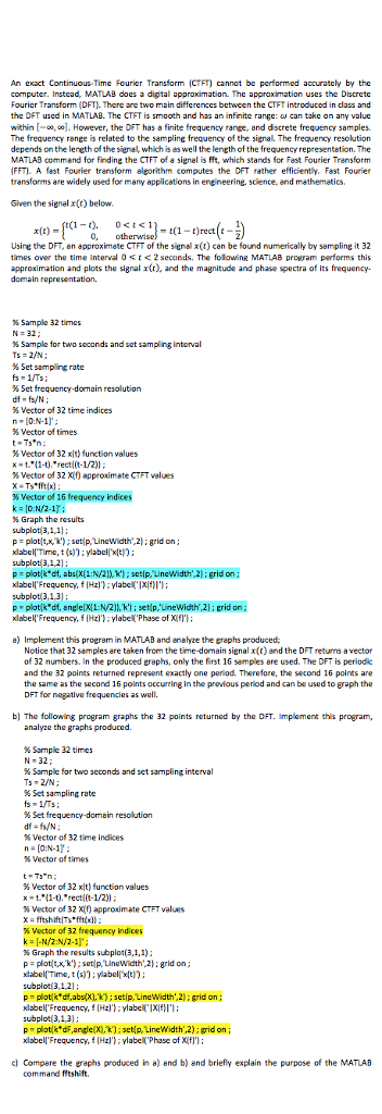
% Sample 32 times N = 32 ; % Sample for two seconds and set sampling interval Ts = 2/N ; % Set sampling rate fs = 1/Ts ; % Set frequency-domain resolution df = fs/N ; % Vector of 32 time indices n = [0:N-1]' ; % Vector of times t = Ts*n ; % Vector of 32 x(t) function values x = t.*(1-t).*rect((t-1/2)) ; % Vector of 32 X(f) approximate CTFT values X = Ts*fft(x) ; % Vector of 16 frequency indices k = [0:N/2-1]' ; % Graph the results subplot(3,1,1) ; p = plot(t,x,'k') ; set(p,'LineWidth',2) ; grid on ; xlabel('Time, t (s)') ; ylabel('x(t)') ; subplot(3,1,2) ; p = plot(k*df, abs(X(1:N/2)),'k') ; set(p,'LineWidth',2) ; grid on ; xlabel('Frequency, f (Hz)') ; ylabel('|X(f)|') ; subplot(3,1,3) ; p = plot(k*df, angle(X(1:N/2)),'k') ; set(p,'LineWidth',2) ; grid on ; xlabel('Frequency, f (Hz)') ; ylabel('Phase of X(f)') ;

FOR PART B)

% Sample 32 times N = 32 ; % Sample for two seconds and set sampling interval Ts = 2/N ; % Set sampling rate fs = 1/Ts ; % Set frequency-domain resolution df = fs/N ; % Vector of 32 time indices n = [0:N-1]' ; % Vector of times ELEC 242 Continuous-Time Signals & Systems Summer 2017 Department of Electrical & Computer Engineering - Concordia University Dr. Abdelaziz Trabelsi Page 3/3 t = Ts*n ; % Vector of 32 x(t) function values x = t.*(1-t).*rect((t-1/2)) ; % Vector of 32 X(f) approximate CTFT values X = fftshift(Ts*fft(x)) ; % Vector of 32 frequency indices k = [-N/2:N/2-1]' ; % Graph the results subplot(3,1,1) ; p = plot(t,x,'k') ; set(p,'LineWidth',2) ; grid on ; xlabel('Time, t (s)') ; ylabel('x(t)') ; subplot(3,1,2) ; p = plot(k*df,abs(X),'k') ; set(p,'LineWidth',2) ; grid on ; xlabel('Frequency, f (Hz)') ; ylabel('|X(f)|') ; subplot(3,1,3) ; p = plot(k*dF,angle(X),'k') ; set(p,'LineWidth',2) ; grid on ; xlabel('Frequency, f (Hz)') ; ylabel('Phase of X(f)') ;

An exact Continuous-Time Fourier Transform (CTFT) cannot be performed accurately by the computer. Instead, MATLAB does a digital approximation. The approximation uses the Discrete Fourier Transform (DFT). There are two main differences between the CTFT introduced in class and the DFT used in MATLAB. The CTFT is smooth and has an in infinite range:omega can take on any value within [-infinity, infinity]. However, the DFT has a finite frequency range, and discrete frequency samples. The frequency range is related to the sampling frequency of the signal. The frequency resolution depends on the length of the signal, which is as well the length of the frequency representation. The MATLAB command for finding the CTFT of a signal is fft, which stands for Fast Fourier Transform (FFT). A fast Fourier transform algorithm computes the DFT rather efficiently. Fast Fourier transforms are widely used for many application in engineering, science, and mathematics. Given the signal x(t) below. x(t) = { t(1 - t), 0