MATLAB QUESTION:

Please do the entire question if possible, I mainly need help with b) but you need to do a) to get b).

Please provide the code that was modified also.

Thank you.

File Name: DirectionalField.m

function [ ] = DirectionField( X_min, X_max, X_step, Y_min, Y_max, Y_step )

%DirectionField:: This function is a slight modification of

% the function SlopeFlied.

% This function allows us to plot the

% direction field of a first order 2-dimensional differential equation

% given by the function H(x,y).

%

% There is no output for this function. The input variables are as

% follows:

%X_min : The minimum x-value in our graph.

%X_max : The maximum x-value in our graph.

%X_step : The spacing in 'x' between the slope lines.

%Y_min : The minimum y-value in our graph.

%Y_max : The maximum y-value in our graph.

%Y_step : The spacing in 'y' between the slope lines.

% This function creates a matrix X and a matrix Y

%

[X,Y] = meshgrid(X_min:X_step:X_max,Y_min:Y_step:Y_max);

% We want to create a vector field, with vectors located at the points

% designated by the matricies X and Y.

% To that end, we create two new matrices 'rise' and 'run' which are the

% same size as X.

% 'rise' will contain the y-component of each vector

% 'run' will contain the x-component of each vector

rise=X;

run =X;

% We create a loop which will iterate over the coordinates (i,j) inside our

% matrices 'rise' and 'run'

for i = 1:length(rise(:,1))

for j = 1:length(rise(1,:))

% First we calculate the x & y values of the point in the graph

x = X(i,j);

y = Y(i,j);

% Now we calculate the function H(x,y).

[ Delta_X , Delta_Y] = H(x,y);

% We calculate the vector norm of ( Delta_T , Delta_Y )

Norm = sqrt( Delta_X^2 + Delta_Y^2 );

% We store the normalized vector.

% If we didn't do this, we'd just have a vector field.

rise(i,j) = Delta_Y / Norm;

run(i,j) = Delta_X / Norm;

end

end

% Using the function 'quiver', we produce our direction field!

quiver(X,Y,run,rise)

% We add on the labels 'X' and 'Y' onto the x and y axes respectively

xlabel('X')

ylabel('Y')

end

File Name: ExampleDirectionField.m

%%% This file uses the following matlab files

%%% H.m

%%% DirectionField.m

%%%

%%% This file will plot the direction field of the 2-dimensional

%%% differential equation

%%% (x',y') = H(x,y).

% We clear all variables which may have been defined

clear

% These variables define the minimum and maximum values

% for "X" in the direction field.

X_min = -3;

X_max = 3;

% These variables define the minimum and maximum values

% for "Y" in the direction field.

Y_min = -3;

Y_max = 3;

% These variables define the spacings between the slope lines

% in the X and Y directions.

X_step = 1;

Y_step = 1;

% This creates a new figure window and plots the direction field

figure

DirectionField( X_min, X_max, X_step, Y_min, Y_max, Y_step )

File name: H.m

function [ x_derivative , y_derivative ] = H( x, y )

% The function "H" is used to define

% a first order 2-dimensional differential equation.

% x' = x_derivative

% y' = y_derivative

% By default, we use the differential equation

% x' = y;

% y' = x - x^3 -y^3;

x_derivative = y;

y_derivative = x - x^3 -y^3;

end

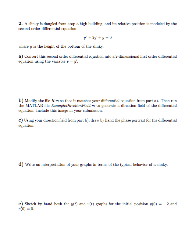
2. A slinky is dangled from atop a high building, and its relative position is modeled by the second order differential equation where y is the height of the bottom of the slinky. a) Convert this second order differential equation into a 2-dimensional first order differential equation using the variable v b) Modify the file H.m so that it matches your differential equation from part a). Then run the MATLAB file EzampleDirectionField.m to generate a direction field of the differential equation. Include this image in your submission. c) Using your direction field from part b), draw by hand the phase portrait for the differential equation. d) Write an interpretation of your graphs in terms of the typical behavior of a slinky. e) Sketch by hand both the y(t) and v(t) graphs for the initial position y (0) 2 and