%matplotlib inline

import matplotlib.pyplot as plt

import numpy as np

from scipy.special import binom

from scipy.optimize import least_squares

np.seterr(over='raise')

def StoneMod(Rtot, Kd, v, Kx, L0):

'''

Returns the number of mutlivalent ligand bound to a cell with Rtot

receptors, granted each epitope of the ligand binds to the receptor

kind in question with dissociation constant Kd and cross-links with

other receptors with crosslinking constant Kx. All eq derived from Stone et al. (2001).

'''

v = np.int_(v)

assert L0.shape == v.shape

# Mass balance for receptor species, to identify the amount of free receptor

diffFunAnon = lambda x: Rtot-x*(1+v*L0*(1/Kd)*(1+Kx*x)**(v-1))

## Solve Req by calling least_squares

lsq = least_squares(diffFunAnon, np.full_like(L0, Rtot/2.0), jac_sparsity=np.eye(L0.size),

max_nfev=1000, xtol=1.0E-10, ftol=1.0E-10, gtol=1.0E-10,

bounds=(np.full_like(L0, -np.finfo(float).eps), np.full_like(L0, Rtot)))

if lsq['cost'] > 1.0E-8:

print(lsq)

raise RuntimeError("Failure in solving for Req.")

Req = lsq.x

Lbound = np.zeros(Req.size)

Rmulti = np.zeros(Req.size)

Rbnd = np.zeros(Req.size)

for ii, Reqq in enumerate(Req):

# Calculate vieq from equation 1

vieq = L0[ii]*Reqq*binom(v[ii], np.arange(1, v[ii] + 1))*np.power(Kx*Reqq, np.arange(v[ii]))/Kd

# Calculate L, according to equation 7

Lbound[ii] = np.sum(vieq)

# Calculate Rmulti from equation 5

Rmulti[ii] = np.dot(vieq[1:], np.arange(2, v[ii] + 1, dtype=np.float))

# Calculate Rbound

Rbnd[ii] = Rmulti[ii] + vieq[0]

return (Lbound, Rbnd, Rmulti)

Xs = np.array([8.1E-11, 3.4E-10, 1.3E-09, 5.7E-09, 2.1E-08, 8.7E-08, 3.4E-07, 1.5E-06, 5.7E-06, 2.82E-11, 1.17E-10, 4.68E-10, 1.79E-09, 7.16E-09, 2.87E-08, 1.21E-07, 4.5E-07, 1.87E-06, 1.64E-11, 6.93E-11, 2.58E-10, 1.11E-09, 4.35E-09, 1.79E-08, 7.38E-08, 2.9E-07, 1.14E-06])

Ys = np.array([-196, -436, 761, 685, 3279, 7802, 11669, 12538, 9012, -1104, -769, 1455, 2693, 7134, 11288, 14498, 16188, 13237, 988, 1734, 4491, 9015, 13580, 17159, 18438, 18485, 17958])

Vs = np.repeat([2, 3, 4], 9)

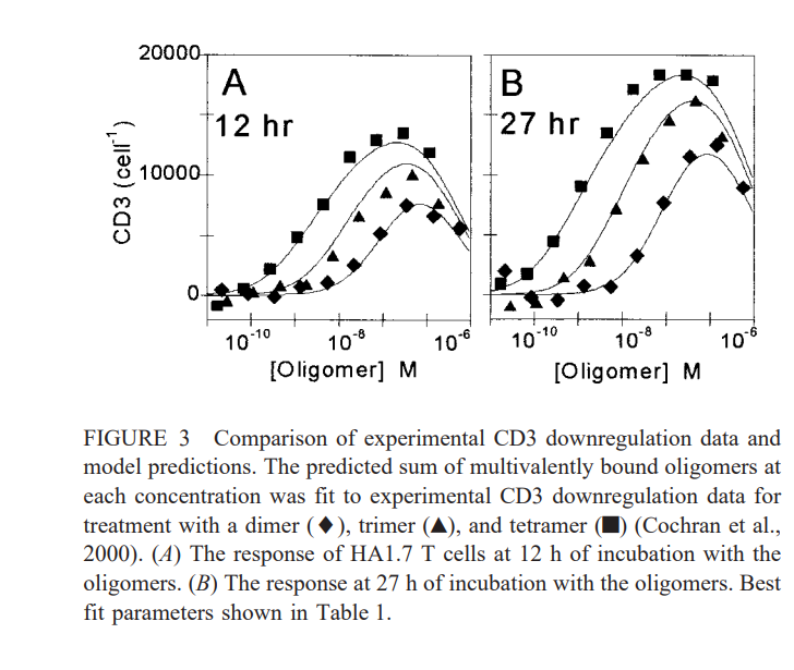
#### We will fit the data contained within Fig. 3B. Plot this data and describe the relationship you see between Kx, Kd, and valency. Python.

FIGURE 3 Comparison of experimental CD3 downregulation data and model predictions. The predicted sum of multivalently bound oligomers at each concentration was fit to experimental CD3 downregulation data for treatment with a dimer (), trimer (), and tetramer ( ) (Cochran et al., 2000). (A) The response of HA1.7 T cells at 12h of incubation with the oligomers. (B) The response at 27h of incubation with the oligomers. Best fit parameters shown in Table 1