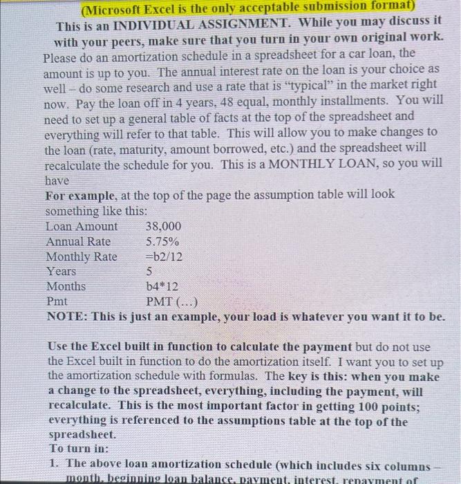
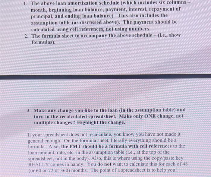
(Microsoft Excel is the only acceptable submission format) This is an INDIVIDUAL ASSIGNMENT. While you may discuss it with your peers, make sure that you turn in your own original work. Please do an amortization schedule in a spreadsheet for a car loan, the amount is up to you. The annual interest rate on the loan is your choice as well - do some research and use a rate that is "typical" in the market right now. Pay the loan off in 4 years, 48 equal, monthly installments. You will need to set up a general table of facts at the top of the spreadsheet and everything will refer to that table. This will allow you to make changes to the loan (rate, maturity, amount borrowed, etc.) and the spreadsheet will recalculate the schedule for you. This is a MONTHLY LOAN, so you will have For example, at the top of the page the assumption table will look something like this: NU1E: Ihis is just an example, your load is whatever you want it to be. Use the Excel built in function to calculate the payment but do not use the Excel built in function to do the amortization itself. I want you to set up the amortization schedule with formulas. The key is this: when you make a change to the spreadsheet, everything, including the payment, will recalculate. This is the most important factor in getting 100 points; everything is referenced to the assumptions table at the top of the spreadsheet. To turn in: 1. The above loan amortization schedule (which includes six columns - 1. The above loan amortization schedule (which includes six columns month, beginning loan balance, payment, interest, repayment of principal, and ending loan balance). This also includes the assumption table (as discussed above). The payment should be calculated using cell references, not using numbers. 2. The formula sheet to accompany the above schedule - (i.e., show formulas). 3. Make any change you like to the loan (in the assumption table) and turn in the recalculated spreadsheet. Make only ONE change, not multiple changes!! Highlight the change. If your spreadsheet does not recalculate, you know you have not made it general enough. On the formula sheet, literally everything should be a formula. Also, the PMT should be a formula with cell references to the loan amount, rate, etc. in the assumption table (i.e., at the top of the spreadsheet, not in the body). Also, this is where using the copy/paste key REAILY comes in handy. You do not want to calculate this for each of 48 (or 60 or 72 or 360 ) months. The point of a spreadsheet is to help you


