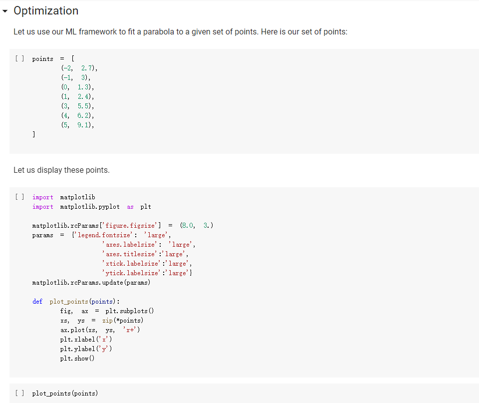
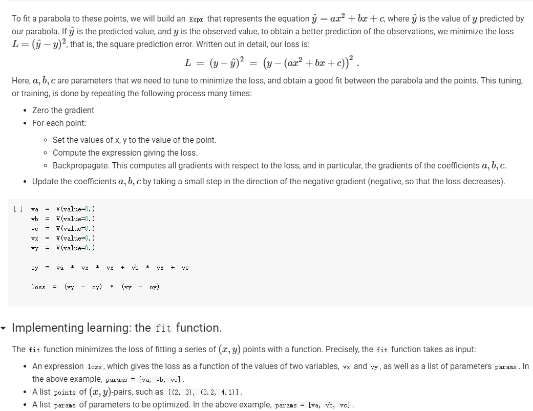
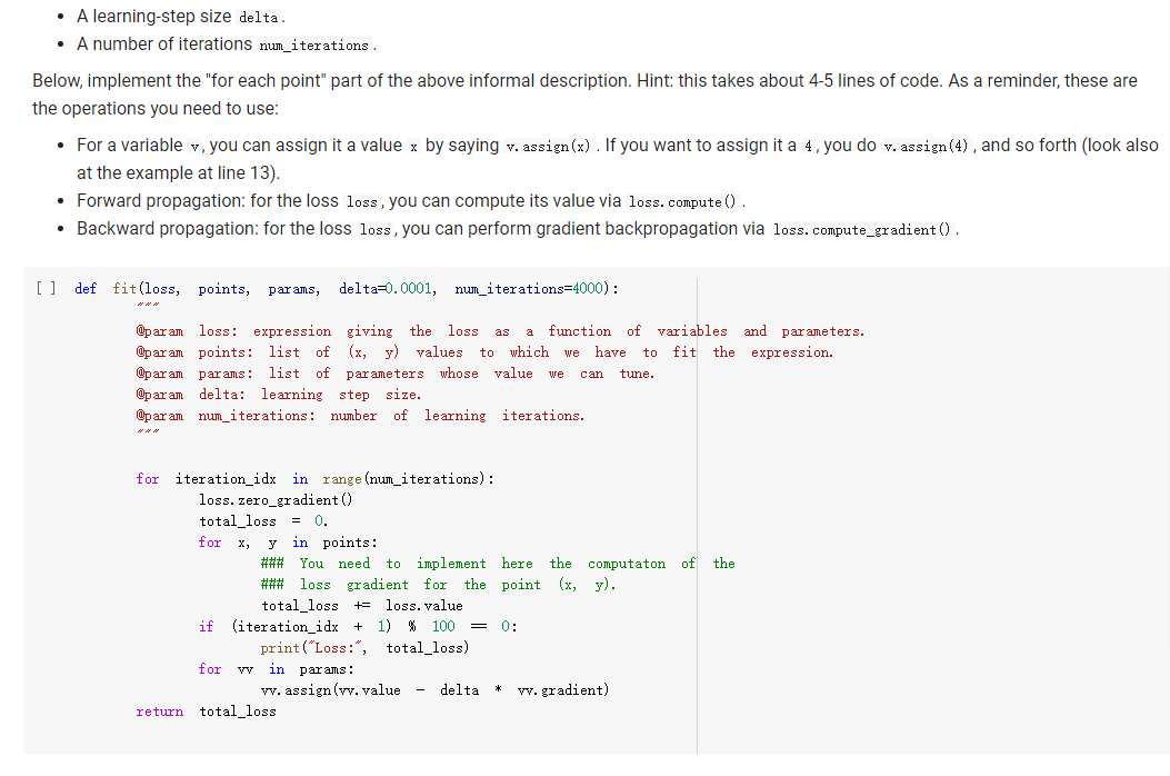
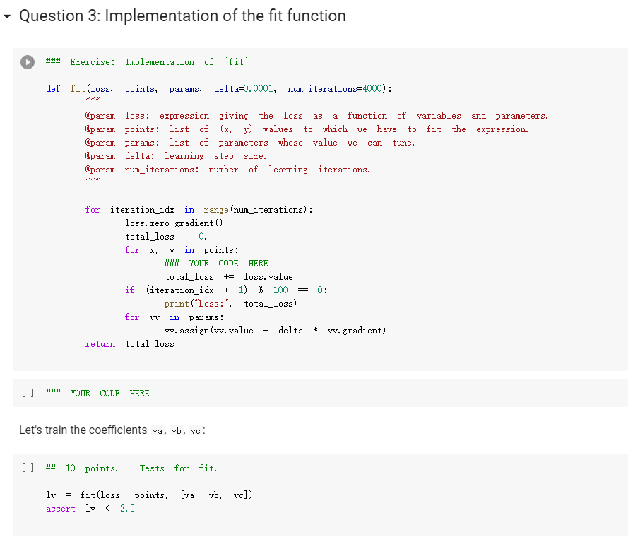
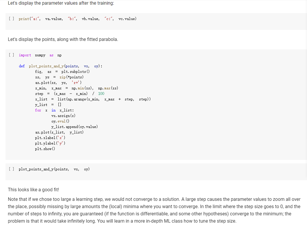
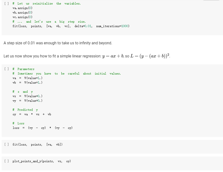
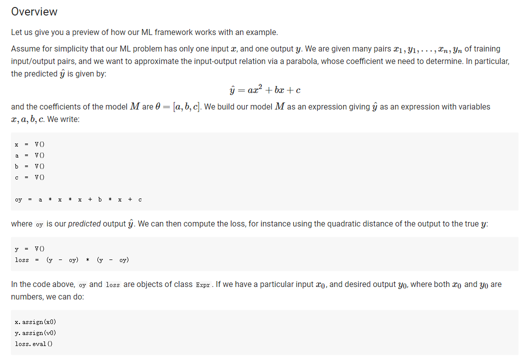
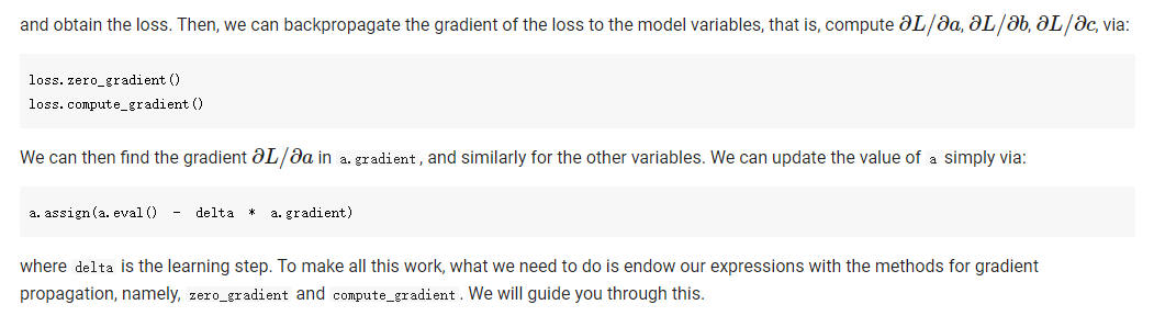
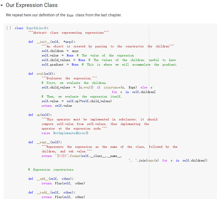
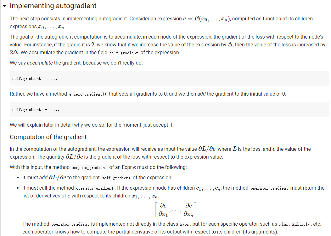
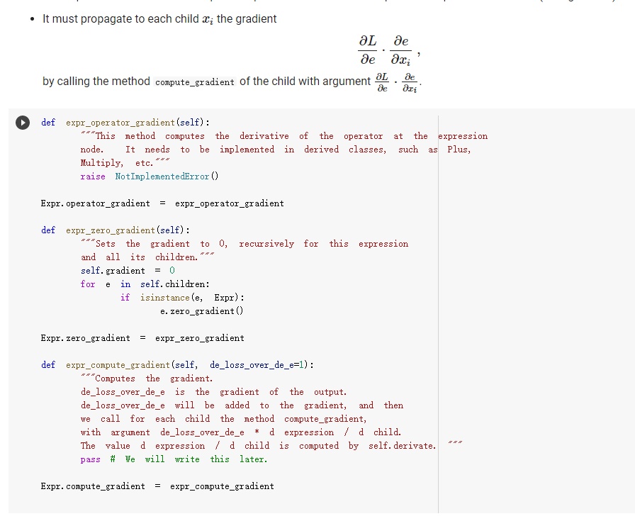
ML in a nutshell Optimization, and machine learning, are intimately connected. At a very coarse level, ML works as follows. First, you come up somehow with a very complicated model y = M(x, 0), which computes an output y as a function of an input x and of a vector of parameters 0. In general, x, y, and are vectors, as the model has multiple inputs, multiple outputs, and several parameters. The model M needs to be complicated, because only complicated models can represent complicated phenomena; for instance, M can be a multi- layer neural net with parameters 0 = (01,..., Ok], where k is the number of parameters of the model. Second, you come up with a notion of loss L, that is, how badly the model is doing. For instance, if you have a list of inputs X1,...,n, and a set of desired outputs y1, ..., ym, you can use as loss: L(0) =&gs - I =) lyi MX1,0). i=1 Here, we wrote L(0) because, once the inputs 11,..., In and the desired outputs yi, ..., Yn are chosen, the loss L depends only on 0. Once the loss is chosen, you decrease it, by computing its gradient with respect to 0. Remembering that 0 = [01,...,0k) [ al al VAL= ai ak The gradient is a vector that indicates how to tweak 0 to decrease the loss. You then choose a small step size 8, and you update via 0:= 0 - 8V L. This makes the loss a little bit smaller, and the model a little bit better. If you repeat this step many times, the model will hopefully get a good bit) better. Autogradient The key to pleasant ML is to focus on building the model M in a way that is sufficiently expressive, and on choosing a loss L that is helpful in guiding the optimization. The computation of the gradient is done automatically for you. This capability, called autogradient, is implemented in ML frameworks such as Tensorflow, Keras, and Py Torch. It is possible to use these advanced ML libraries without ever knowing what is under the hood, and how autogradient works. Here, we will insted dive in, and implement autogradient. Building a model M corresponds to building an expression with inputs x, 0. We will provide a representaton for expressions that enables both the calculation of the expression value, and the differentiation with respect to any of the inputs. This will enable us to implement autogradient. On the basis of this, we will be able to implement a simple ML framework. We say we, but we mean you. You will implement it; we will just provide guidance. Overview Let us give you a preview of how our ML framework works with an example. Assume for simplicity that our ML problem has only one input x, and one output y. We are given many pairs 21, 41, ..., xn, yn of training input/output pairs, and we want to approximate the input-output relation via a parabola, whose coefficient we need to determine. In particular, the predicted is given by: ax2 + bx+c and the coefficients of the model Mare 0 = [a,b,c). We build our model M as an expression giving as an expression with variables x, a, b, c. We write: VO) = V() b = = oy * x + b * x + c where oy is our predicted output . We can then compute the loss, for instance using the quadratic distance of the output to the true y: y = VO) loss (y - oy) = * (y - oy) In the code above, oy and loss are objects of class Expr. If we have a particular input xo, and desired output yo, where both 2o and yo are numbers, we can do: x. assign (x0) y. assign (vo) loss. eval() and obtain the loss. Then, we can backpropagate the gradient of the loss to the model variables, that is, compute alaa, al ab, al/ac, via: loss. zero_gradient() loss. compute_gradient We can then find the gradient ala in a. gradient, and similarly for the other variables. We can update the value of a simply via: a. assign(a. eval() delta * a. gradient) where delta is the learning step. To make all this work, what we need to do is endow our expressions with the methods for gradient propagation, namely, zero_gradient and compute_gradient. We will guide you through this. , Our Expression Class We repeat here our definition of the Expr class from the last chapter. [] class Expr (object): "Abstract class representing expressions def __init__(self, *args) : An object is created by passing to the constructor the children self.children args self.value = None # The value of the expression self.child_values None # The values of the children: useful to have self. gradient = None # This is where will accumulate the gradient. = we we def eval(self): ***Evaluates the expression. # First, evaluate the children. self.child_values = [c. eval() if isinstance(c, Expr) else c for in self.children] # Then, evaluate the expression itself. self.value = self.op(*self.child_values) return self.value we def op (self): "This operator must be implemented in subclasses; it should compute self.value from self.values, thus implementing the operator at the expression node. raise NotImplementedError() def name of the class, followed by the -repr -_(self): ***Represents the expression as the children, and teh value. return "{} ({})". format (self._class_ name ?. join (repr (c) for c in self.children)) # Expression constructors def _add_(self, other): return Plus (self, other) def _radd_(self, other): return Plus (self, other) def _radd__(self, other): return Plus(self, other) def _sub_(self, other): return Minus (self, other) def _rsub_(self, other): return Minus (other, self) def _mul_(self, other): return Multiply(self, other) def _rmul_(self, other): Multiply (other, self) return def _truediv_(self, other): return Divide (self, other) def _r truediv_(self, other): return Divide (other, self) def _neg__(self): return Negative (self) [] import random import string class V(Expr): ***Variable. *** def _init__(self, value=None): super(). _init_o self.children = self.value = random. gauss (0, 1) if value is None else value self.name random. choices (string, ascii_letters + string. digits, k=8)) = ''. join def eval(self): return self.value def assign(self, value): self.value = value 84 10- self.value value def _repr_(self): return "v(name={}, value={})". format (self.name, self.value) [] class Plus (Expr): def op (self, return x, y): X + Y class Minus (Expr): def op (self, return x, y): class Multiply(Expr): def op (self, return X, * class Divide (Expr): def op (self, return x, y): x / y class Negative (Expr): def op(self, x): return [ ] = V(value=3) V(value=2) = - vy assert e. eval() 1. Implementing autogradient The next step consists in implementing autogradient. Consider an expression e = E(20,..., In), computed as function of its children expressions 20, ..., In The goal of the autogradient computation is to accumulate, in each node of the expression, the gradient of the loss with respect to the node's value. For instance, if the gradient is 2, we know that if we increase the value of the expression by A, then the value of the loss is increased by 2A. We accumulate the gradient in the field self. gradient of the expression. We say accumulate the gradient, because we don't really do: self. gradient = Rather, we have a method e.zero_gradient() that sets all gradients to 0, and we then add the gradient to this initial value of 0: self. gradient + We will explain later in detail why we do so; for the moment, just accept it. Computaton of the gradient In the computation of the autogradient, the expression will receive as input the value a/de, where L is the loss, and e the value of the expression. The quantity alfae is the gradient of the loss with respect to the expression value. With this input, the method compute_gradient of an Expr e must do the following: It must add alae to the gradient self. gradient of the expression. It must call the method operator_gradient. If the expression node has children C1,..., Cr, the method operator_gradient must return the list of derivatives of e with respect to its children 21,...,ni ae ae axi arn The method operator_gradient is implemented not directly in the class Expr, but for each specific operator, such as Plus, Multiply, etc: each operator knows how to compute the partial derivative of its output with respect to its children (its arguments). It must propagate to each child &; the gradient al ae ; al by calling the method compute_gradient of the child with argument dri 7 de def expr_operator_gradient (self): ***This method computes the derivative of the operator at the expression node. It needs to be implemented in derived classes, such as Plus, Multiply, etc. raise NotImplementedError() Expr. operator_gradient expr_operator_gradient def expr_zero_gradient (self): Sets the gradient to 0, recursively for this expression and all its children. self. gradient = 0 for in self.children: if isinstance(e, Expr): e. zero_gradient() Expr. zero_gradient = expr_zero_gradient def expr_compute_gradient (self, de_loss_over_de_e=1): ***Computes the gradient. de_loss_over_de_e is the gradient of the output. de_loss_over_de_e will be added to the gradient, and then call for each child the method compute_gradient, with argument de_loss_over_de_e * d expression / d child. The value d expression / d child is computed by self. derivate. pass # We will write this later. we Expr. compute_gradient = expr_compute_gradient Let us endow our classes Plus and Multiply with the operator_gradient method, so you can see how it works in practice. [] def plus_operator_gradient (self): # If e = x + y, de / dx = return 1, 1 1, and de 1 dy = 1 Plus. operator_gradient = plus_operator_gradient and de / dy = x def multiply operator_gradient(self): # If e = x * y, de / dx = y, y = self.child_values return y X Multiply. operator_gradient = multiply_operator_gradient def variable_operator_gradient(self): # This is not really used, but it needs return None to be here for completeness. V. operator_gradient = variable_operator_gradient Let us comment on some subtle points, before you get to work at implementing compute_gradient. zero_gradient: First, notice how in the implementation of zero_gradient, when we loop over the children, we check whether each children is an Expr via isinstance(e, Expr). In general, we have to remember that children can be either Expr, or simply numbers, and of course numbers do not have methods such as zero_gradient or compute_gradient implemented for them. operator_gradient: Second, notice how operator_gradient is not implemented in Expr directly, but rather, only in the derived classes such as Plus. The derivative of the expression with respect to its arguments depends on which function it is, obviously. For Plus, we have e = xo + 21, and so: ae =1 =1, a.co axi because d(x+y) dx =1. Hence, the operator_gradient method of Plus returns ae [1,1] | For Multiply, we have e = co.21, and so: ae ae = 21 axi because d(xy) /dx = y. Hence, the operator_gradient method of Plus returns [1,20]. axo' axi =101 = Calling compute before compute_gradient: Lastly, a very important point: when calling compute_gradient, we will assume that eval has already been called. In this way, the value of the expression, and its children, are available for the computation of the gradient. Note how in Multiply. derivate we use these values in order to compute the partial derivatives. Question 1 With these clarifications, we ask you to implement the compute_gradient method, which again must: add al de to the gradient self. gradient of the expression; compute doen by calling the method operator_gradient of itself; propagate to each child X; the gradient al.de, by calling the method compute_gradient of the child i with argument OL zi de dri ### Exercise: Implementation of compute_gradient to def expr_compute_gradient (self, de_loss_over_de_e=1): ***Computes the gradient. de_loss_over_de_e is the gradient of the output. de_loss_over_de_e will be added the gradient, and then we call for each child the method compute_gradient, with argument de_loss_over_de_e * d expression / d child. The valued expression / d child is computed by self. derivate. ### YOUR CODE HERE Expr. compute_gradient = expr_compute_gradient [] ### YOUR CODE HERE Below are some tests. [] ## Tests for compute_gradient a SLUIL . VX VZ = + VZ # First, the gradient of = V(value=3) V(value=) y assert y. eval() 7 y. zero_gradient() y. compute_gradient() assert vx. gradient 1 a product. VZ = # Second, the gradient of = V(value=3) V(value=4) Y VZ assert y. eval() 12 y. zero_gradient() y. compute_gradient() assert vx. gradient 4 assert vz. gradient 3 # Finally, the gradient of the product of SUMS. VX = VW = VZ V(value=1) V(value=3) = V(value=4) Y (vx + vw) assert y. eval() y. zero_gradient() y.compute_gradient() assert vx. gradient assert vz. gradient (vz + 3) 28 = = 7 4 [] ### Hidden tests for compute gradient Why do we accumulate gradients? We are now in the position of answering the question of why we accumulate gradients. There are two reasons. Multiple variable occurrence The most important reason why we need to add to the gradient of each node is that nodes, and in particular, variable nodes, can occur in multiple places in an expression tree. To compute the total influence of the variable on the expression, we need to sum the influence of each occurrence. Let's see this with a simple example. Consider the expression y=x.x. We can code it as follows: [ ] VX # Creates a variable VX and initializes it to 2. = V(2.) = * y vX For y=x?, we have dy/dx = 2x = 4, given that x =2. How is this reflected in our code? Our code considers separately the left and right occurrences of vx in the expression; let us Val and var expression can be written as y=vxl VXF, and we have that ay a vx1 = VI, = 2, as var = 2. Similarly, ay a vzr = 2. These two gradients are added to vx. gradient by the method compute_gradient, and we get that the total gradient is 4, as desired. [] y. eval() # We have to call eval() before compute_gradient() y. zero_gradient() y.compute_gradient() print(" gradient of vx:", vx. gradient) assert vx. gradient = 4 Multiple data to fit The other reason why we need to tally up the gradient is that in general, we need to fit a function to more than one data point. Assume that we are given a set of inputs 21, 22, ..., Un and desired outputs y1, y2, ..., Yn. Our goal is to approximate the desired ouputs via an expression y=e(a,0) of the input, according to some parameters 0. Our goal is to choose the parameters 0 to minimize the sum of the square errors for the points: Luz (0) = L(0) =fe(25,6) u.), where L;(O) = (elli, 0) yi)2 is the loss for a single data point. The gradient Ltot () with respect to can be computed by adding up the gradients for the individual points: a Ltot (0) ae ae a L;O) To translate this into code, we will build an expression e(x, 0) involving the input x and the parameters 0, and an expression L=(e(x, 0) y)2 for the loss, involving x, y and 0. We will then zero all gradients via zero_gradient. Once this is done, we compute the loss L for each point (Li, Yi), and then the gradient al/ae via a call to compute_gradient. The gradients for all the points will be added, yielding the gradient for minimizing the total loss over all the points. Question 2: Rounding up the implementation Now that we have implemented autogradient, as well as the operators Plus and Multiply, it is time to implement the remaining operators: Minus Divide (no need to worry about division by zero) and the unary minus Negative. [] ### Exercise: Implementation of Minus, Divide, and "Negative def minus_operator_gradient (self): # Ife = x - y, de / dx = ### YOUR CODE HERE and de / dy = Minus. operator_gradient = minus_operator_gradient def divide_operator_gradient (self): # If e = x/y, de / dx = ### YOUR CODE HERE .. and de / dy = ... [] ### YOUR CODE HERE Divide. operator_gradient = divide_operator_gradient def negative_operator_gradient (self): # If e = -X, de / dx = ... ### YOUR CODE HERE Negative. operator_gradient = negative_operator_gradient [] ### YOUR CODE HERE Here are some tests. ### Tests for Minus = = # Minus. V(value=3) V(value=2) e vX - Vy ssert e. eval() e. zero_gradient() e.compute_gradient() assert vx. gradient assert vy.gradient 1. = 1 = -1 [] ### Hidden tests for Minus [ ] # Tests for Divide e # Divide. = V(6) V(2) vx / vy assert e. eval() e. zero_gradient() e. compute_gradient() assert vx. gradient assert vy. gradient 3 0.5 -1.5 [] ### Hidden tests for Divide [] ## Tests for Negative Negative VX = = VX assert e. eval() e. zero_gradient() e.compute_gradient() assert vx. gradient -1 [ ] ### Hidden tests for Negative Optimization Let us use our ML framework to fit a parabola to a given set of points. Here is our set of points: [ ] points = [ (-2, 2.7), (-1, 3), O, 1.3), (1, 2. 4), (3, 5.5), (4, 5.2), (5, 9.1), ] Let us display these points. [ ] import matplotlib import matplotlib.pyplot as plt 3 matplotlib.rcParams['figure.figsize'] = (8.0, 3.) params ['legend. fontsize': 'large', axes. labelsize': 'large', axes. titlesize':'large', 'xtick. labelsize' :' large', 'ytick. labelsize':'large'} matplotlib.rcParams. update (params) ax = def plot_points (points): fig, plt. subplotso) XS, ys zip(*points) ax.plot(x, ys, 'r+') plt. xlabel('x') plt. ylabel('y) plt.show() [] plot_points (points) + c))? To fit a parabola to these points, we will build an Expr that represents the equation = ax+ bx+c, where y is the value of y predicted by our parabola. If is the predicted value, and y is the observed value, to obtain a better prediction of the observations, we minimize the loss L= ( - y)2, that is, the square prediction error. Written out in detail, our loss is: L = (y- y)2 = (y (ax? +be+ Here, a, b, c are parameters that we need to tune to minimize the loss, and obtain a good fit between the parabola and the points. This tuning, or training, is done by repeating the following process many times: Zero the gradient For each point: o Set the values of x,y to the value of the point. o Compute the expression giving the loss. Backpropagate. This computes all gradients with respect to the loss, and in particular, the gradients of the coefficients a, b, c. Update the coefficients a, b, c by taking a small step in the direction of the negative gradient (negative, so that the loss decreases). [] va vb VC = V(value=0.) = V(value=0.) = V(value=0.) = V(value=0.) = V(value=0.) oy = va * * + vb * vx + VC loss = (vy - oy) ** oy) Implementing learning: the fit function. The fit function minimizes the loss of fitting a series of (x, y) points with a function. Precisely, the fit function takes as input: An expression loss, which gives the loss as a function of the values of two variables, vx and vy, as well as a list of parameters params . In the above example, params = [va, vb, vc]. A list points of (x,y)-pairs, such as [(2, 3), (3.2, 4.1)]. A list params of parameters to be optimized. In the above example, params = [va, vb, vc]. A learning-step size delta. A number of iterations num_iterations. Below, implement the "for each point" part of the above informal description. Hint: this takes about 4-5 lines of code. As a reminder, these are the operations you need to use: For a variable y, you can assign it a value x by saying v. assign(x). If you want to assign it a 4, you do v. assign(4), and so forth (look also at the example at line 13). Forward propagation: for the loss loss, you can compute its value via loss. compute(). Backward propagation: for the loss loss, you can perform gradient backpropagation via loss.compute_gradient(). [] def fit(loss, points, params, delta=0.0001, num_iterations=4000): @param loss: expression giving the loss as a function of variables and parameters. @param points: list of (x, y) values to which we have to fit the expression. @param params: list of parameters whose value we can tune. @param delta: learning step size. param num_iterations: number of learning iterations. the for iteration_idx in range(num_iterations): loss. zero_gradient() total_loss = 0. for x, y in points: ### You need to implement here the computaton of ### loss gradient for the point (x, y). total_loss loss. value if (iteration_idx + 1) % 100 = 0: print("Loss:", total_loss) for in params: w. assign (vv.value delta * w.gradient) return total_loss + Question 3: Implementation of the fit function ### Exercise: Implementation of 'fit def fit(loss, points, params, delta=0.0001, num_iterations=4000): as we @param loss: expression giving the loss a function of variables and parameters. @param points: list of (x, y) values to which have to fit the expression. @param tune. params: list of parameters whose value @param delta: learning step size. @param num_iterations: number of learning iterations. we can for iteration_idx in range(num_iterations): loss. zero_gradient() total_loss 0. for X, y in points: ### YOUR CODE HERE total_loss += loss. value if (iteration_idx + 1) % 100 0: print("Loss:", total_loss) for v in params: w. assign(vv. value delta * v. gradient) return total_loss = [] ### YOUR CODE HERE Let's train the coefficients va, vb, vc: [] ## 10 points. Tests for fit. ly vc]) fit(loss, points, [va, vb, ly ( 3. 5 assert Let's display the parameter values after the training: [ ] print("a", va. value, "B:", vb. value, "c:", vc. value) Let's display the points, along with the fitted parabola. [] import numpy as np = + step, step)) def plot_points_and_y (points, VX, oy): fig, ax plt. subplots() Xs, y = zip(*points) ax.plot(xs, ys, 'It') x_min, x_max = np. min(xs), np. max(xs) step (x_max - x_min) / 100 x_list list (np. arange(x_min, x_max y_list = [] for in x_list: vx. assign(x) oy. eval() y_list. append(oy. value) ax.plot(x_list, y_list) plt. xlabel('x') plt. ylabel('y) plt.show() X [ ] plot_points_and_y (points, vx, oy) This looks like a good fit! Note that if we chose too large a learning step, we would not converge to a solution. A large step causes the parameter values to zoom all over the place, possibly missing by large amounts the (local) minima where you want to converge. In the limit where the step size goes to 0, and the number of steps to infinity, you are guaranteed (if the function is differentiable, and some other hypotheses) converge to the minimum; the problem is that it would take infinitely long. You will learn in a more in-depth ML class how to tune the step size. [] # Let us reinitialize the variables. va assign (0) vb. assign (0) vc. assign (0) # ... and let's a big step size. fit(loss, points, [va, vb, vc], delta=0.01, num_iterations=1000) use A step size of 0.01 was enough to take us to infinity and beyond. Let us now show you how to fit a simple linear regression: y = ax +b, so L =(y-ax+b))2. to be careful about initial values. [ ] # Parameters # Sometimes you have = V(value=1.) vb = V(value=1.) va and y = V(value=0.) V(value=0.) = # Predicted y oy VX + vb # Loss loss (vy oy) (vy oy) [] fit(loss, points, [va, vb]) [] plot_points_and_y (points, VX; oy) ML in a nutshell Optimization, and machine learning, are intimately connected. At a very coarse level, ML works as follows. First, you come up somehow with a very complicated model y = M(x, 0), which computes an output y as a function of an input x and of a vector of parameters 0. In general, x, y, and are vectors, as the model has multiple inputs, multiple outputs, and several parameters. The model M needs to be complicated, because only complicated models can represent complicated phenomena; for instance, M can be a multi- layer neural net with parameters 0 = (01,..., Ok], where k is the number of parameters of the model. Second, you come up with a notion of loss L, that is, how badly the model is doing. For instance, if you have a list of inputs X1,...,n, and a set of desired outputs y1, ..., ym, you can use as loss: L(0) =&gs - I =) lyi MX1,0). i=1 Here, we wrote L(0) because, once the inputs 11,..., In and the desired outputs yi, ..., Yn are chosen, the loss L depends only on 0. Once the loss is chosen, you decrease it, by computing its gradient with respect to 0. Remembering that 0 = [01,...,0k) [ al al VAL= ai ak The gradient is a vector that indicates how to tweak 0 to decrease the loss. You then choose a small step size 8, and you update via 0:= 0 - 8V L. This makes the loss a little bit smaller, and the model a little bit better. If you repeat this step many times, the model will hopefully get a good bit) better. Autogradient The key to pleasant ML is to focus on building the model M in a way that is sufficiently expressive, and on choosing a loss L that is helpful in guiding the optimization. The computation of the gradient is done automatically for you. This capability, called autogradient, is implemented in ML frameworks such as Tensorflow, Keras, and Py Torch. It is possible to use these advanced ML libraries without ever knowing what is under the hood, and how autogradient works. Here, we will insted dive in, and implement autogradient. Building a model M corresponds to building an expression with inputs x, 0. We will provide a representaton for expressions that enables both the calculation of the expression value, and the differentiation with respect to any of the inputs. This will enable us to implement autogradient. On the basis of this, we will be able to implement a simple ML framework. We say we, but we mean you. You will implement it; we will just provide guidance. Overview Let us give you a preview of how our ML framework works with an example. Assume for simplicity that our ML problem has only one input x, and one output y. We are given many pairs 21, 41, ..., xn, yn of training input/output pairs, and we want to approximate the input-output relation via a parabola, whose coefficient we need to determine. In particular, the predicted is given by: ax2 + bx+c and the coefficients of the model Mare 0 = [a,b,c). We build our model M as an expression giving as an expression with variables x, a, b, c. We write: VO) = V() b = = oy * x + b * x + c where oy is our predicted output . We can then compute the loss, for instance using the quadratic distance of the output to the true y: y = VO) loss (y - oy) = * (y - oy) In the code above, oy and loss are objects of class Expr. If we have a particular input xo, and desired output yo, where both 2o and yo are numbers, we can do: x. assign (x0) y. assign (vo) loss. eval() and obtain the loss. Then, we can backpropagate the gradient of the loss to the model variables, that is, compute alaa, al ab, al/ac, via: loss. zero_gradient() loss. compute_gradient We can then find the gradient ala in a. gradient, and similarly for the other variables. We can update the value of a simply via: a. assign(a. eval() delta * a. gradient) where delta is the learning step. To make all this work, what we need to do is endow our expressions with the methods for gradient propagation, namely, zero_gradient and compute_gradient. We will guide you through this. , Our Expression Class We repeat here our definition of the Expr class from the last chapter. [] class Expr (object): "Abstract class representing expressions def __init__(self, *args) : An object is created by passing to the constructor the children self.children args self.value = None # The value of the expression self.child_values None # The values of the children: useful to have self. gradient = None # This is where will accumulate the gradient. = we we def eval(self): ***Evaluates the expression. # First, evaluate the children. self.child_values = [c. eval() if isinstance(c, Expr) else c for in self.children] # Then, evaluate the expression itself. self.value = self.op(*self.child_values) return self.value we def op (self): "This operator must be implemented in subclasses; it should compute self.value from self.values, thus implementing the operator at the expression node. raise NotImplementedError() def name of the class, followed by the -repr -_(self): ***Represents the expression as the children, and teh value. return "{} ({})". format (self._class_ name ?. join (repr (c) for c in self.children)) # Expression constructors def _add_(self, other): return Plus (self, other) def _radd_(self, other): return Plus (self, other) def _radd__(self, other): return Plus(self, other) def _sub_(self, other): return Minus (self, other) def _rsub_(self, other): return Minus (other, self) def _mul_(self, other): return Multiply(self, other) def _rmul_(self, other): Multiply (other, self) return def _truediv_(self, other): return Divide (self, other) def _r truediv_(self, other): return Divide (other, self) def _neg__(self): return Negative (self) [] import random import string class V(Expr): ***Variable. *** def _init__(self, value=None): super(). _init_o self.children = self.value = random. gauss (0, 1) if value is None else value self.name random. choices (string, ascii_letters + string. digits, k=8)) = ''. join def eval(self): return self.value def assign(self, value): self.value = value 84 10- self.value value def _repr_(self): return "v(name={}, value={})". format (self.name, self.value) [] class Plus (Expr): def op (self, return x, y): X + Y class Minus (Expr): def op (self, return x, y): class Multiply(Expr): def op (self, return X, * class Divide (Expr): def op (self, return x, y): x / y class Negative (Expr): def op(self, x): return [ ] = V(value=3) V(value=2) = - vy assert e. eval() 1. Implementing autogradient The next step consists in implementing autogradient. Consider an expression e = E(20,..., In), computed as function of its children expressions 20, ..., In The goal of the autogradient computation is to accumulate, in each node of the expression, the gradient of the loss with respect to the node's value. For instance, if the gradient is 2, we know that if we increase the value of the expression by A, then the value of the loss is increased by 2A. We accumulate the gradient in the field self. gradient of the expression. We say accumulate the gradient, because we don't really do: self. gradient = Rather, we have a method e.zero_gradient() that sets all gradients to 0, and we then add the gradient to this initial value of 0: self. gradient + We will explain later in detail why we do so; for the moment, just accept it. Computaton of the gradient In the computation of the autogradient, the expression will receive as input the value a/de, where L is the loss, and e the value of the expression. The quantity alfae is the gradient of the loss with respect to the expression value. With this input, the method compute_gradient of an Expr e must do the following: It must add alae to the gradient self. gradient of the expression. It must call the method operator_gradient. If the expression node has children C1,..., Cr, the method operator_gradient must return the list of derivatives of e with respect to its children 21,...,ni ae ae axi arn The method operator_gradient is implemented not directly in the class Expr, but for each specific operator, such as Plus, Multiply, etc: each operator knows how to compute the partial derivative of its output with respect to its children (its arguments). It must propagate to each child &; the gradient al ae ; al by calling the method compute_gradient of the child with argument dri 7 de def expr_operator_gradient (self): ***This method computes the derivative of the operator at the expression node. It needs to be implemented in derived classes, such as Plus, Multiply, etc. raise NotImplementedError() Expr. operator_gradient expr_operator_gradient def expr_zero_gradient (self): Sets the gradient to 0, recursively for this expression and all its children. self. gradient = 0 for in self.children: if isinstance(e, Expr): e. zero_gradient() Expr. zero_gradient = expr_zero_gradient def expr_compute_gradient (self, de_loss_over_de_e=1): ***Computes the gradient. de_loss_over_de_e is the gradient of the output. de_loss_over_de_e will be added to the gradient, and then call for each child the method compute_gradient, with argument de_loss_over_de_e * d expression / d child. The value d expression / d child is computed by self. derivate. pass # We will write this later. we Expr. compute_gradient = expr_compute_gradient Let us endow our classes Plus and Multiply with the operator_gradient method, so you can see how it works in practice. [] def plus_operator_gradient (self): # If e = x + y, de / dx = return 1, 1 1, and de 1 dy = 1 Plus. operator_gradient = plus_operator_gradient and de / dy = x def multiply operator_gradient(self): # If e = x * y, de / dx = y, y = self.child_values return y X Multiply. operator_gradient = multiply_operator_gradient def variable_operator_gradient(self): # This is not really used, but it needs return None to be here for completeness. V. operator_gradient = variable_operator_gradient Let us comment on some subtle points, before you get to work at implementing compute_gradient. zero_gradient: First, notice how in the implementation of zero_gradient, when we loop over the children, we check whether each children is an Expr via isinstance(e, Expr). In general, we have to remember that children can be either Expr, or simply numbers, and of course numbers do not have methods such as zero_gradient or compute_gradient implemented for them. operator_gradient: Second, notice how operator_gradient is not implemented in Expr directly, but rather, only in the derived classes such as Plus. The derivative of the expression with respect to its arguments depends on which function it is, obviously. For Plus, we have e = xo + 21, and so: ae =1 =1, a.co axi because d(x+y) dx =1. Hence, the operator_gradient method of Plus returns ae [1,1] | For Multiply, we have e = co.21, and so: ae ae = 21 axi because d(xy) /dx = y. Hence, the operator_gradient method of Plus returns [1,20]. axo' axi =101 = Calling compute before compute_gradient: Lastly, a very important point: when calling compute_gradient, we will assume that eval has already been called. In this way, the value of the expression, and its children, are available for the computation of the gradient. Note how in Multiply. derivate we use these values in order to compute the partial derivatives. Question 1 With these clarifications, we ask you to implement the compute_gradient method, which again must: add al de to the gradient self. gradient of the expression; compute doen by calling the method operator_gradient of itself; propagate to each child X; the gradient al.de, by calling the method compute_gradient of the child i with argument OL zi de dri ### Exercise: Implementation of compute_gradient to def expr_compute_gradient (self, de_loss_over_de_e=1): ***Computes the gradient. de_loss_over_de_e is the gradient of the output. de_loss_over_de_e will be added the gradient, and then we call for each child the method compute_gradient, with argument de_loss_over_de_e * d expression / d child. The valued expression / d child is computed by self. derivate. ### YOUR CODE HERE Expr. compute_gradient = expr_compute_gradient [] ### YOUR CODE HERE Below are some tests. [] ## Tests for compute_gradient a SLUIL . VX VZ = + VZ # First, the gradient of = V(value=3) V(value=) y assert y. eval() 7 y. zero_gradient() y. compute_gradient() assert vx. gradient 1 a product. VZ = # Second, the gradient of = V(value=3) V(value=4) Y VZ assert y. eval() 12 y. zero_gradient() y. compute_gradient() assert vx. gradient 4 assert vz. gradient 3 # Finally, the gradient of the product of SUMS. VX = VW = VZ V(value=1) V(value=3) = V(value=4) Y (vx + vw) assert y. eval() y. zero_gradient() y.compute_gradient() assert vx. gradient assert vz. gradient (vz + 3) 28 = = 7 4 [] ### Hidden tests for compute gradient Why do we accumulate gradients? We are now in the position of answering the question of why we accumulate gradients. There are two reasons. Multiple variable occurrence The most important reason why we need to add to the gradient of each node is that nodes, and in particular, variable nodes, can occur in multiple places in an expression tree. To compute the total influence of the variable on the expression, we need to sum the influence of each occurrence. Let's see this with a simple example. Consider the expression y=x.x. We can code it as follows: [ ] VX # Creates a variable VX and initializes it to 2. = V(2.) = * y vX For y=x?, we have dy/dx = 2x = 4, given that x =2. How is this reflected in our code? Our code considers separately the left and right occurrences of vx in the expression; let us Val and var expression can be written as y=vxl VXF, and we have that ay a vx1 = VI, = 2, as var = 2. Similarly, ay a vzr = 2. These two gradients are added to vx. gradient by the method compute_gradient, and we get that the total gradient is 4, as desired. [] y. eval() # We have to call eval() before compute_gradient() y. zero_gradient() y.compute_gradient() print(" gradient of vx:", vx. gradient) assert vx. gradient = 4 Multiple data to fit The other reason why we need to tally up the gradient is that in general, we need to fit a function to more than one data point. Assume that we are given a set of inputs 21, 22, ..., Un and desired outputs y1, y2, ..., Yn. Our goal is to approximate the desired ouputs via an expression y=e(a,0) of the input, according to some parameters 0. Our goal is to choose the parameters 0 to minimize the sum of the square errors for the points: Luz (0) = L(0) =fe(25,6) u.), where L;(O) = (elli, 0) yi)2 is the loss for a single data point. The gradient Ltot () with respect to can be computed by adding up the gradients for the individual points: a Ltot (0) ae ae a L;O) To translate this into code, we will build an expression e(x, 0) involving the input x and the parameters 0, and an expression L=(e(x, 0) y)2 for the loss, involving x, y and 0. We will then zero all gradients via zero_gradient. Once this is done, we compute the loss L for each point (Li, Yi), and then the gradient al/ae via a call to compute_gradient. The gradients for all the points will be added, yielding the gradient for minimizing the total loss over all the points. Question 2: Rounding up the implementation Now that we have implemented autogradient, as well as the operators Plus and Multiply, it is time to implement the remaining operators: Minus Divide (no need to worry about division by zero) and the unary minus Negative. [] ### Exercise: Implementation of Minus, Divide, and "Negative def minus_operator_gradient (self): # Ife = x - y, de / dx = ### YOUR CODE HERE and de / dy = Minus. operator_gradient = minus_operator_gradient def divide_operator_gradient (self): # If e = x/y, de / dx = ### YOUR CODE HERE .. and de / dy = ... [] ### YOUR CODE HERE Divide. operator_gradient = divide_operator_gradient def negative_operator_gradient (self): # If e = -X, de / dx = ... ### YOUR CODE HERE Negative. operator_gradient = negative_operator_gradient [] ### YOUR CODE HERE Here are some tests. ### Tests for Minus = = # Minus. V(value=3) V(value=2) e vX - Vy ssert e. eval() e. zero_gradient() e.compute_gradient() assert vx. gradient assert vy.gradient 1. = 1 = -1 [] ### Hidden tests for Minus [ ] # Tests for Divide e # Divide. = V(6) V(2) vx / vy assert e. eval() e. zero_gradient() e. compute_gradient() assert vx. gradient assert vy. gradient 3 0.5 -1.5 [] ### Hidden tests for Divide [] ## Tests for Negative Negative VX = = VX assert e. eval() e. zero_gradient() e.compute_gradient() assert vx. gradient -1 [ ] ### Hidden tests for Negative Optimization Let us use our ML framework to fit a parabola to a given set of points. Here is our set of points: [ ] points = [ (-2, 2.7), (-1, 3), O, 1.3), (1, 2. 4), (3, 5.5), (4, 5.2), (5, 9.1), ] Let us display these points. [ ] import matplotlib import matplotlib.pyplot as plt 3 matplotlib.rcParams['figure.figsize'] = (8.0, 3.) params ['legend. fontsize': 'large', axes. labelsize': 'large', axes. titlesize':'large', 'xtick. labelsize' :' large', 'ytick. labelsize':'large'} matplotlib.rcParams. update (params) ax = def plot_points (points): fig, plt. subplotso) XS, ys zip(*points) ax.plot(x, ys, 'r+') plt. xlabel('x') plt. ylabel('y) plt.show() [] plot_points (points) + c))? To fit a parabola to these points, we will build an Expr that represents the equation = ax+ bx+c, where y is the value of y predicted by our parabola. If is the predicted value, and y is the observed value, to obtain a better prediction of the observations, we minimize the loss L= ( - y)2, that is, the square prediction error. Written out in detail, our loss is: L = (y- y)2 = (y (ax? +be+ Here, a, b, c are parameters that we need to tune to minimize the loss, and obtain a good fit between the parabola and the points. This tuning, or training, is done by repeating the following process many times: Zero the gradient For each point: o Set the values of x,y to the value of the point. o Compute the expression giving the loss. Backpropagate. This computes all gradients with respect to the loss, and in particular, the gradients of the coefficients a, b, c. Update the coefficients a, b, c by taking a small step in the direction of the negative gradient (negative, so that the loss decreases). [] va vb VC = V(value=0.) = V(value=0.) = V(value=0.) = V(value=0.) = V(value=0.) oy = va * * + vb * vx + VC loss = (vy - oy) ** oy) Implementing learning: the fit function. The fit function minimizes the loss of fitting a series of (x, y) points with a function. Precisely, the fit function takes as input: An expression loss, which gives the loss as a function of the values of two variables, vx and vy, as well as a list of parameters params . In the above example, params = [va, vb, vc]. A list points of (x,y)-pairs, such as [(2, 3), (3.2, 4.1)]. A list params of parameters to be optimized. In the above example, params = [va, vb, vc]. A learning-step size delta. A number of iterations num_iterations. Below, implement the "for each point" part of the above informal description. Hint: this takes about 4-5 lines of code. As a reminder, these are the operations you need to use: For a variable y, you can assign it a value x by saying v. assign(x). If you want to assign it a 4, you do v. assign(4), and so forth (look also at the example at line 13). Forward propagation: for the loss loss, you can compute its value via loss. compute(). Backward propagation: for the loss loss, you can perform gradient backpropagation via loss.compute_gradient(). [] def fit(loss, points, params, delta=0.0001, num_iterations=4000): @param loss: expression giving the loss as a function of variables and parameters. @param points: list of (x, y) values to which we have to fit the expression. @param params: list of parameters whose value we can tune. @param delta: learning step size. param num_iterations: number of learning iterations. the for iteration_idx in range(num_iterations): loss. zero_gradient() total_loss = 0. for x, y in points: ### You need to implement here the computaton of ### loss gradient for the point (x, y). total_loss loss. value if (iteration_idx + 1) % 100 = 0: print("Loss:", total_loss) for in params: w. assign (vv.value delta * w.gradient) return total_loss + Question 3: Implementation of the fit function ### Exercise: Implementation of 'fit def fit(loss, points, params, delta=0.0001, num_iterations=4000): as we @param loss: expression giving the loss a function of variables and parameters. @param points: list of (x, y) values to which have to fit the expression. @param tune. params: list of parameters whose value @param delta: learning step size. @param num_iterations: number of learning iterations. we can for iteration_idx in range(num_iterations): loss. zero_gradient() total_loss 0. for X, y in points: ### YOUR CODE HERE total_loss += loss. value if (iteration_idx + 1) % 100 0: print("Loss:", total_loss) for v in params: w. assign(vv. value delta * v. gradient) return total_loss = [] ### YOUR CODE HERE Let's train the coefficients va, vb, vc: [] ## 10 points. Tests for fit. ly vc]) fit(loss, points, [va, vb, ly ( 3. 5 assert Let's display the parameter values after the training: [ ] print("a", va. value, "B:", vb. value, "c:", vc. value) Let's display the points, along with the fitted parabola. [] import numpy as np = + step, step)) def plot_points_and_y (points, VX, oy): fig, ax plt. subplots() Xs, y = zip(*points) ax.plot(xs, ys, 'It') x_min, x_max = np. min(xs), np. max(xs) step (x_max - x_min) / 100 x_list list (np. arange(x_min, x_max y_list = [] for in x_list: vx. assign(x) oy. eval() y_list. append(oy. value) ax.plot(x_list, y_list) plt. xlabel('x') plt. ylabel('y) plt.show() X [ ] plot_points_and_y (points, vx, oy) This looks like a good fit! Note that if we chose too large a learning step, we would not converge to a solution. A large step causes the parameter values to zoom all over the place, possibly missing by large amounts the (local) minima where you want to converge. In the limit where the step size goes to 0, and the number of steps to infinity, you are guaranteed (if the function is differentiable, and some other hypotheses) converge to the minimum; the problem is that it would take infinitely long. You will learn in a more in-depth ML class how to tune the step size. [] # Let us reinitialize the variables. va assign (0) vb. assign (0) vc. assign (0) # ... and let's a big step size. fit(loss, points, [va, vb, vc], delta=0.01, num_iterations=1000) use A step size of 0.01 was enough to take us to infinity and beyond. Let us now show you how to fit a simple linear regression: y = ax +b, so L =(y-ax+b))2. to be careful about initial values. [ ] # Parameters # Sometimes you have = V(value=1.) vb = V(value=1.) va and y = V(value=0.) V(value=0.) = # Predicted y oy VX + vb # Loss loss (vy oy) (vy oy) [] fit(loss, points, [va, vb]) [] plot_points_and_y (points, VX; oy)