Moving Average Excel
you will need this info to compute
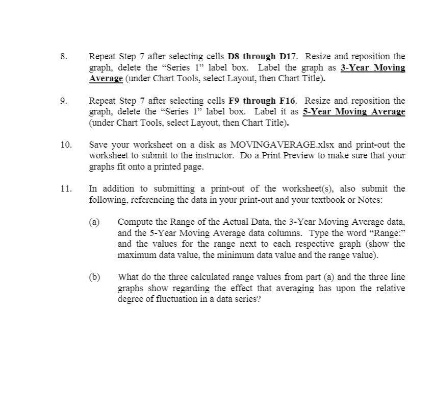
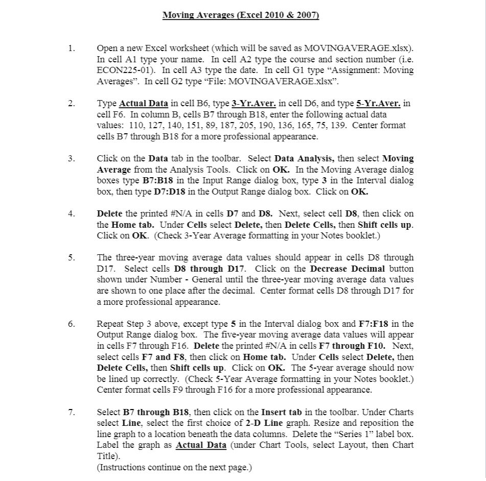
M0 ' Av es ccl 2.010 8; 200 Open a new Excel worksheet (which will be saved as MDVRGGAVERAGExlsx}. In cell Al type your name. In cell A2 type the course and section number (i.e. ECON225-01). In cell A3 type the date. In cell G1 type \"Assignment: Moving Averages\". In cell G2 type \"File: MOVRQGAVERAGExlsx\". Type Actual Data in cell 36, type 3-Yr.Aver. in cell D6, and type 5Yr.Avcr. in cell F6. In column B, cells B7 through B 13, enter the following actual data values: 110, 127, 1411, 151, 89, 187, 205, 190, I36, 165, 75, 139. Center format cells B7 through B 18 for a more professional appearance. Click on the Data tab in the toolbar. Select Data Analysis, then select Moving Average hunt the Analysis Tools. Click on OK. In the Moving Average dialog boxes type B7318 in the Input Range dialog box, type 3 in the Interval dialog box, then type D7:D18 in the Output Range dialog box. Click on OK. Delete the printed #NIA in cells D? and D8. Next, select cell D8, then click on the Home tab. Under Cells select Delete, then Delete Cells, then Shift cells up. Click on OK. (Check 3-Year Average formatting in your Notes booklet.) The three-year moving average data values should appear in cells D3 through D17. Select cells D8 through D17. Click on the Decrease Decimal button shown under Number - General until the three-year moving average data values are shown to one place alter the decimal. Center format cells D3 through D17 for a more professional appearance. Repeat Step 3 above, except type 5 in the Interval dialog box and F7:F18 in the Output Range dialog box. The ve-year moving average data values will appear in cells F7 through F16. Delete the printed #NfA in cells F7 through F10. Next, select cells F7 and F8, then click on Home tab. Under Cells select Delete, then Delete Cells, then Shift cells up. Click on OK. The 5-year average should now be lined up correctly. (filled: 5-Year Average formatting in your Notes booklet.) Center format cells F9 through F16 for a more professional appearance. Select B? through B18, then click on the Insert tab in the toolbar. Under Charts select Line, select the rst choice of 2D Line graph. Resize and reposition the line graph to a location beneath the data columns. Delete the \"Series 1\" label box. 10. 11. Repeat Step '1" after selecting cells D8 through D17. Resize and reposition the graph1 delete the \"Series 1" label box. label the graph as 3Year Moving Average (under Chart Tools= seiect Layout. then Chart Title). Repeat Step 7 after selecting cells F9 through F16. Resize and reposition the graph. delete the \"Series 1\" label box. Label it as 5Year mg g Aveggg (under Chart Tools, select Layout. then Chart Title). Save your worksheet on a disk as MOV'WGAVERAGE.X]5X and print-out the worksheetto submittothe instructor. DoaPrintPreviewtomakesmethatyour graphstontoaprintedpage. In addition to submitting a print-out of the workshees), also submit the following, referencing the data in your print-out and your textbook or Notes: (a) Compute the Range of the Achlal Data. the 3-Year L'Ioving Average data, and the 5-Year Moving Average data columns. Type the word "Range?\" and the values for the range next to each respective graph (Show the maximum data value. the minimum data value and the range value). (b) What do the three calculated range values from part (a) and the three line graphs show regarding the effect that averaging has upon the relative degree of uctuation in a data series


