..Mta 7 help

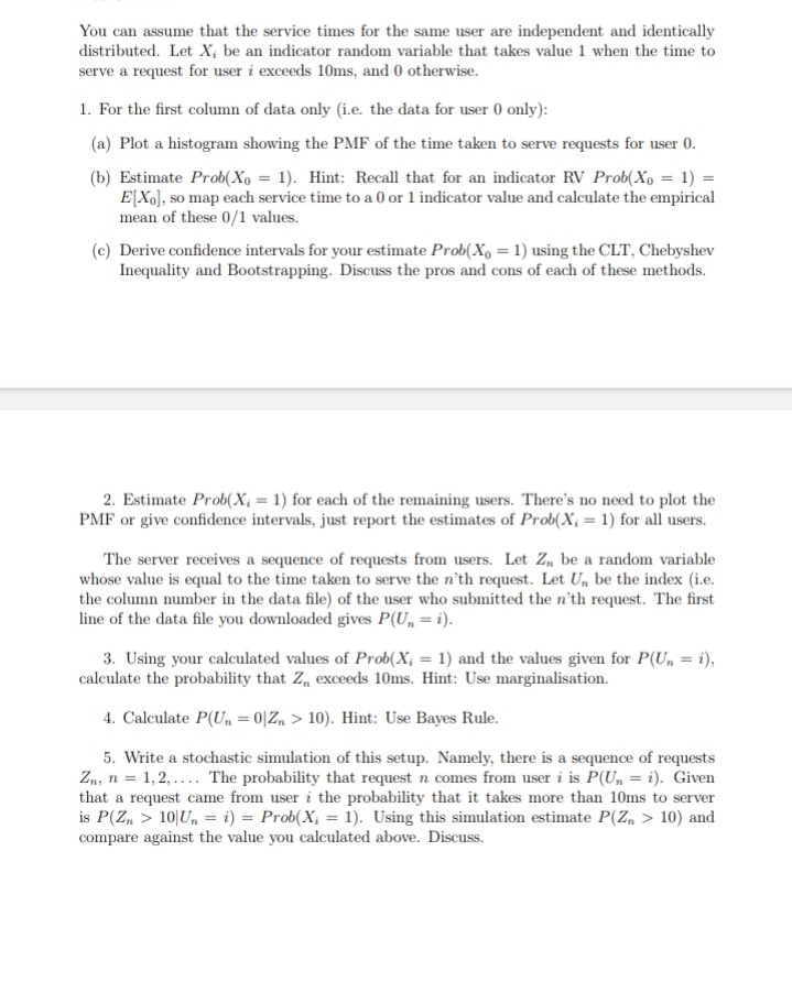
You can assume that the service times for the same user are independent and identically distributed. Let X, be an indicator random variable that takes value 1 when the time to serve a request for user i exceeds 10ms, and 0 otherwise. 1. For the first column of data only (i.e. the data for user 0 only): (a) Plot a histogram showing the PMF of the time taken to serve requests for user 0. (b) Estimate Prob(Xo = 1). Hint: Recall that for an indicator RV Prob(Xo = 1) = E[Xo], so map each service time to a 0 or 1 indicator value and calculate the empirical mean of these 0/1 values. (c) Derive confidence intervals for your estimate Prob(X, = 1) using the CLT, Chebyshev Inequality and Bootstrapping. Discuss the pros and cons of each of these methods. 2. Estimate Prob(X, = 1) for each of the remaining users. There's no need to plot the PMF or give confidence intervals, just report the estimates of Prob(X, = 1) for all users. The server receives a sequence of requests from users. Let Z, be a random variable whose value is equal to the time taken to serve the n'th request. Let U. be the index (i.e. the column number in the data file) of the user who submitted the n'th request. The first line of the data file you downloaded gives P(U, = i). 3. Using your calculated values of Prob(X, = 1) and the values given for P(U,, = i), calculate the probability that Z,, exceeds 10ms. Hint: Use marginalisation. 4. Calculate P(Un = 0|Z, > 10). Hint: Use Bayes Rule. 5. Write a stochastic simulation of this setup. Namely, there is a sequence of requests Zn, n = 1,2,.... The probability that request n comes from user i is P(U, = i). Given that a request came from user i the probability that it takes more than 10ms to server is P(Zn > 10|Un = i) = Prob(X; = 1). Using this simulation estimate P(Z, > 10) and compare against the value you calculated above. Discuss