Answered step by step
Verified Expert Solution
Link Copied!

Question

1 Approved Answer

My main issue is understanding what this assignment is asking me to do and then how to start the project. 5 Interfacing with Blackbox #include
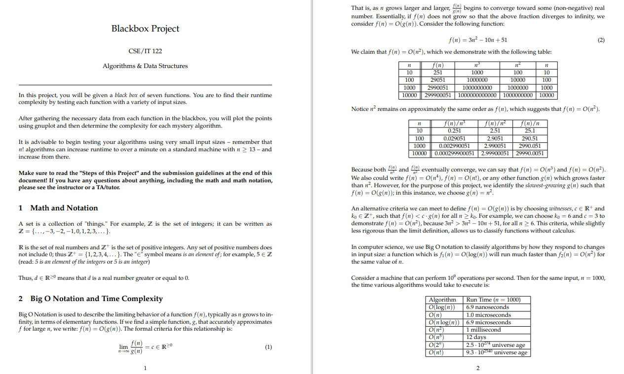
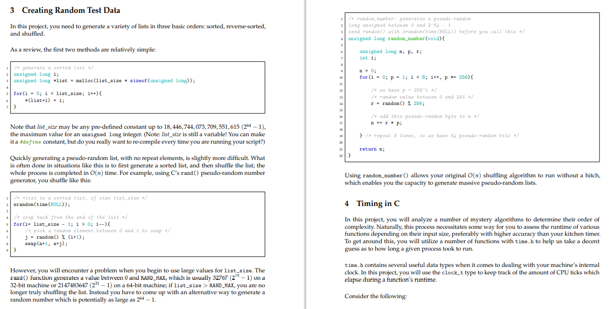
image text in transcribedimage text in transcribedimage text in transcribedimage text in transcribedimage text in transcribedimage text in transcribedimage text in transcribedMy main issue is understanding what this assignment is asking me to do and then how to start the project.

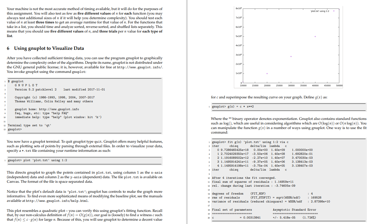
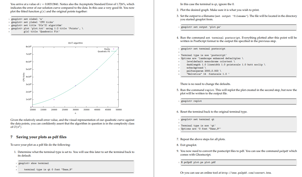
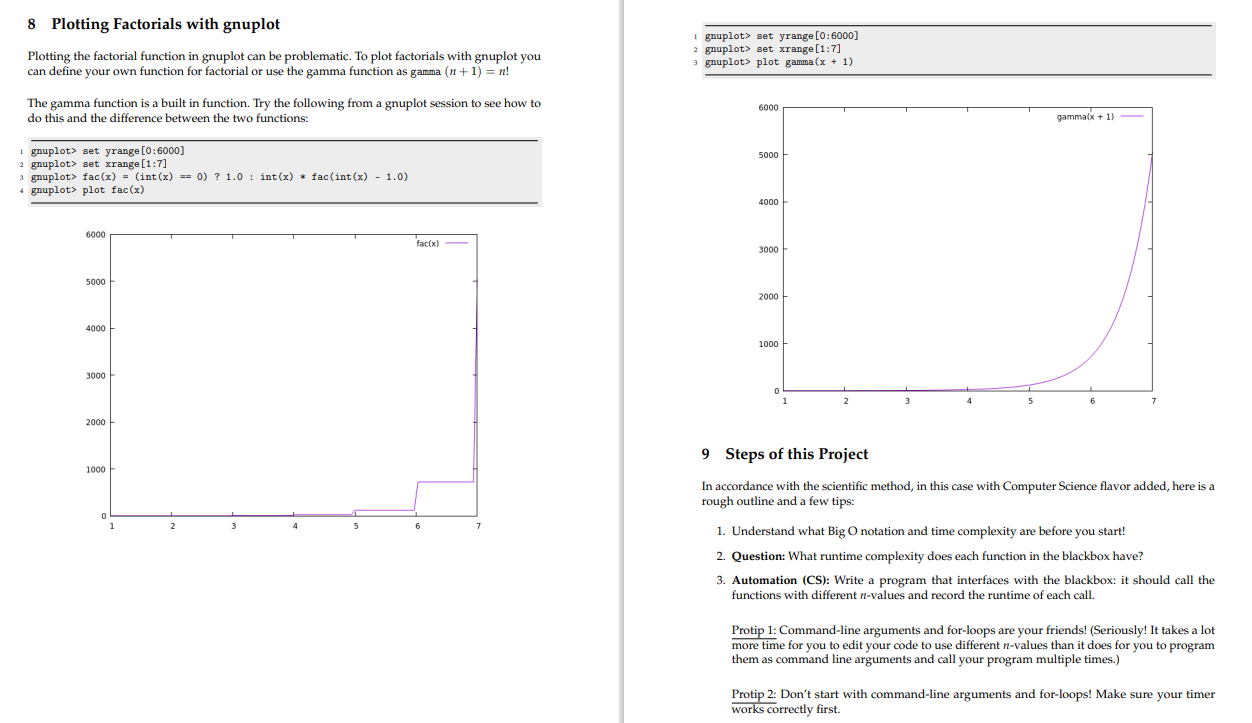
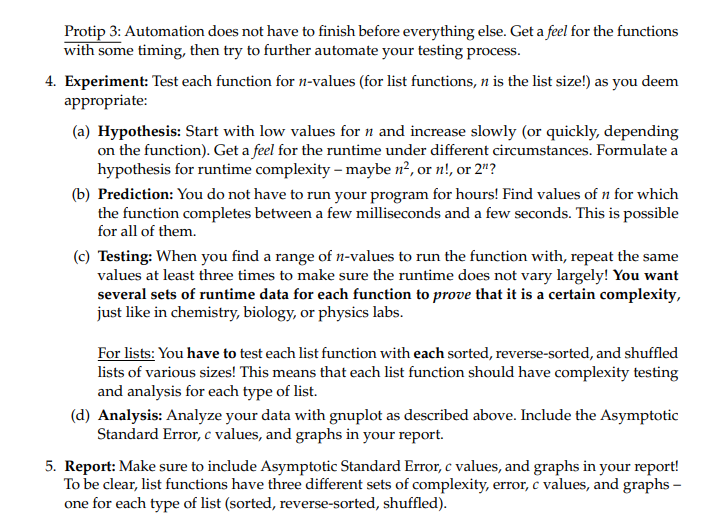
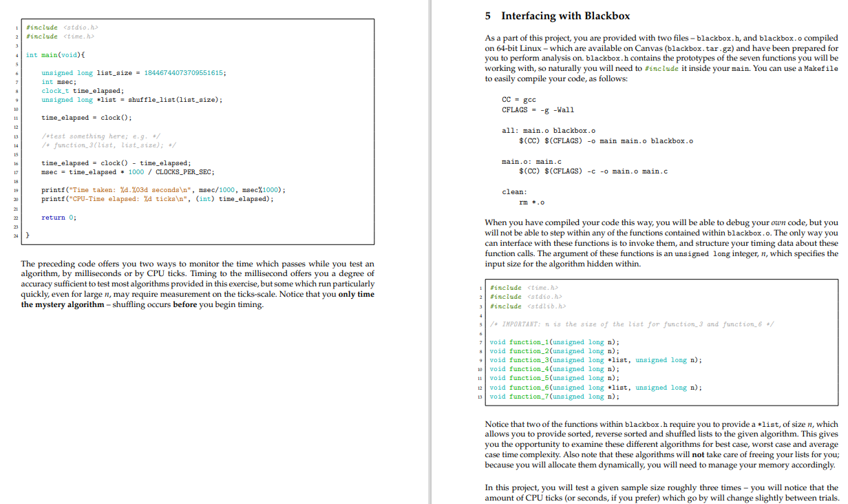
5 Interfacing with Blackbox #include #include 2 3 4 5 int main(void) { As a part of this project, you are provided with two files - blackbox.h, and blackbox.o compiled on 64-bit Linux - which are available on Canvas (blackbox.tar.gz) and have been prepared for you to perform analysis on blackbox.h contains the prototypes of the seven functions you will be working with, so naturally you will need to #include it inside your main. You can use a Makefile to easily compile your code, as follows: 6 unsigned long list_size = 18446744073709551615; int maec; clock_t time_elapsed; unsigned long list = shuffle_list (list_size); 8 9 CC = gcc 10 CFLAGS = -8 -Wall 11 time_elapsed - clock(); 12 13 /*test something here; e.g. */ /* function_3(list, list_size); */ all: main.o blackbox.o $(CC) $ (CFLAGS) - main main.o blackbox.o 14 15 16 time_elapsed = clock() - time_elapsed; msec = time_elapsed - 1000 / CLOCKS_PER_SEC; main.o: main.c $(CC) $ (CFLAGS) -C-o main.o main.c 17 18 printf("Time taken: %0.%03d seconds ", msec/1000, msec%1000); printf("CPU-Time elapsed: %d ticks ", (int) time_elapsed); 21 clean: rm .0 21 22 return 0; 23 24 } When you have compiled your code this way, you will be able to debug your own code, but you will not be able to step within any of the functions contained within blackbox.o. The only way you can interface with these functions is to invoke them, and structure your timing data about these function calls. The argument of these functions is an unsigned long integer, n, which specifies the input size for the algorithm hidden within. The preceding code offers you two ways to monitor the time which passes while you test an algorithm, by milliseconds or by CPU ticks. Timing to the millisecond offers you a degree of accuracy sufficient to test most algorithms provided in this exercise, but some which run particularly quickly, even for large n, may require measurement on the ticks-scale. Notice that you only time the mystery algorithm - shuffling occurs before you begin timing. #include #include #include 3 4 5 /* IMPORTANT: n is the size of the list for function_3 and function_6 */ ? void function_1(unsigned long n); & void function_2(unsigned long n); void function_3(unsigned long list, unsigned long n); 10 void function_4(unsigned long n); 11 void function_5(unsigned long n); 12 void function_6(unsigned long list, unsigned long n); 13 void function_7(unsigned long n); Notice that two of the functions within blackbox.h require you to provide a list of size n, which allows you to provide sorted, reverse sorted and shuffled lists to the given algorithm. This gives you the opportunity to examine these different algorithms for best case, worst case and average case time complexity. Also note that these algorithms will not take care of freeing your lists for you; because you will allocate them dynamically, you will need to manage your memory accordingly. In this project, you will test a given sample size roughly three times - you will notice that the amount of CPU ticks (or seconds, if you prefer) which go by will change slightly between trials. 8x100 plot.txt' using 12 7x10⁶ Your machine is not the most accurate method of timing available, but it will do for the purposes of this assignment. You will also test as few as five different values of n for each function (you may always test additional sizes of n if it will help you determine complexity). You should test each value of n at least three times to get an average runtime for that value of n. For the functions that take in a list, you should time and analyze sorted, reverse-sorted, and shuffled lists separately. This means that you should use five different values of n, and three trials per n value for each type of list. . 6x10⁶ 5x100 4x100 3x10 6 Using gnuplot to Visualize Data After you have collected sufficient timing data, you can use the program gnuplot to graphically determine the complexity order of the algorithms. Despite its name, gnuplot is not distributed under the GNU general public license; it is, however, available for free at http://www.gnuplot.info/. You invoke gnuplot using the command gnuplot: 2x10⁴ 1x10⁶ 0 10000 15000 20000 25000 30000 35000 40000 45000 50000 1 $ gnuplot 2 GNUPLOT 3 Version 5.2 patchlevel 2 last modified 2017-11-01 Copyright (c) 1986-1993, 1998, 2004, 2007-2017 Thomas Williams, Colin Kelley and many others 5 for c and superimpose the resulting curve on your graph. Define g(x) as: 2 1 gnuplot> g(x) = C * x**2 8 gnuplot home: http://www.gnuplot.info 9 faq, bugs, etc: type "help FAQ" 10 immediate help: type "help" (plot window: hit 'h') 11 12 Terminal type set to 'qt' 13 gnuplot> Where the ** binary operator denotes exponentiation. Gnuplot also contains standard functions such as log(), which are useful in considering algorithms which are O(log(n)) or O(n log(n)). You can manipulate the function g(x) in a number of ways using gnuplot. One way is to use the fit command: You now have a gnuplot terminal. To quit gnuplot type quit. Gnuplot offers many helpful features, such as plotting sets of points by parsing through external files. In order to visualize your data, specify a *.txt file containing your runtime information as such: 1 gnuplot> plot 'plot.txt' using 1:2 ' 1 gnuplot> fit g(x) 'plot.txt' using 1:2 viac 2 iter chis delta/lim lambda 3 0 9.7286465425e+18 0.00e+00 1.40e+09 4 1 2.7024029350e+17 -3.50e+06 1.40e+08 + 5 2 1.1916089502e+12 -2.27e+10 1.40e+07 6 3 1.1495914241e+11 -9.37e+05 1.40e+06 4 1.1495914198e+11 -3.75e-04 1.40e+05 8 iter chisa delta/lim lambda 1.000000e+00 1.692820e-01 3.470030e-03 3.138413e-03 3.138407e-03 3 This directs gnuplot to graph the points contained in plot.txt, using column 1 as the x-axis (independent) data and column 2 as the y-axis (dependent) data. The file plot.txt is available on Canvas. The format of the file is space separated data. Notice that the plot's default data is 'plot.txt'; gnuplot has controls to make the graph more informative. To find even more sophisticated means of modifying the baseline plot, see the manuals available at http://www.gnuplot.info/help.html. 10 After 4 iterations the fit converged. 11 final sum of squares of residuals : 1.14959e+11 12 rel. change during last iteration : -3.74605-09 13 14 degrees of freedom (FIT_NDF) 15 rms of residuals (FIT_STDFIT) = sqrt(WSSRdf) 16 variance of residuals (reduced chisquare) = WSSRdf : 169528 : 2.87398e+10 This plot resembles a quadratic plot - you can verify this using gnuplot's fitting function. Recall that, by our non-calculus definition of f(n) =0(8(n)), our goal is (loosely) to find a witness c such that f(n) Sc.8(n) for large n. Because of this, you will use gnuplot to determine a decent value 18 Final set of parameters 19 ======================= 21 C = 0.00313841 Asymptotic Standard Error ================ ======== +/- 5.418e-05 (1.726%) You arrive at a value of c = 0.00313841. Notice also the Asymptotic Standard Error of 1.726%, which indicates the error of our solution curve compared to the data. In this case a very good fit. You now plot the fitted function g(x) and the original points together: In this case the terminal is qt, ignore the 0. 2. Plot the desired graph. Make sure it is what you wish to print. 3. Set the output to a filename set output 'filename'). The file will be located in the directory you started gnuplot from. gnuplot> set xlabel 'n' 2 gnuplot> set ylabel 'CPU ticks 3 gnuplot> set title '0(n-2) algorithm + gnuplot> plot 'plot.txt' using 1:2 title 'Points', \ g(x) title 'Quadratic Fit' gnuplot> set output 'plot.ps' 5 4. Run the command set terminal postscript. Everything plotted after this point will be written in PostScript format to the output file specified in the previous step. On) algorithm Bx106 Points + Quadratic Fit 1 gnuplot> set terminal postscript 2 7x10⁶ 6x100 3 Terminal type is now 'postscript' 4 Options are 'landscape enhanced defaultplex 5 leveldefault monochrome colortext dashlength 1.0 linewidth 1.0 pointscale 1.0 butt noclip 7 nobackground palfuncparam 2000,0.003 "Helvetica" 14 fontacale 1.0 6 5x100 4x100 5 3x10 There is no need to change the defaults. 5. Run the command replot. This will replot the plot created in the second step, but now the plot will be written to the output file. 2x10⁶ 1x10 1 gnuplot> replot 10000 15000 20000 25000 30000 35000 40000 45000 50000 6. Reset the terminal back to the original terminal type. n Given the relatively small error value, and the visual representation of our quadratic curve against the data points, you can confidently assert that the algorithm in question is in the complexity class of O(n). 1 gnuplot> set terminal qt 2 3 Terminal type is now 'qt' + Options are 'O font "Sans,9" 7 Saving your plots as pdf files To save your plot as a pdf file do the following: 7. Repeat the above steps for all plots. 8. Exit gnuplot. 9. You now need to convert the postscript files to pdf. You can use the command ps2pdf which comes with Ghostscript. 1. Determine what the terminal type is set to. You will use this later to set the terminal back to its default. 1 gnuplot> show terminal 1 $ ps2pdf plot.ps plot.pdf 3 terminal type is qt O font "Sans, 9" Or you can use an online tool at http://www.ps2pdf.com/convert.htm. 8 Plotting Factorials with gnuplot Plotting the factorial function in gnuplot can be problematic. To plot factorials with gnuplot you can define your own function for factorial or use the gamma function as gamma (n + 1) = n! 1 gnuplot> set yrange [0:6000] 2 gnuplot> set xrange [1:7] 3 gnuplot> plot gamma (x + 1) The gamma function is a built in function. Try the following from a gnuplot session to see how to do this and the difference between the two functions: 6000 gammalx + 1) 5000 1 gnuplot> set yrange [0:6000) 2 gnuplot> set xrange [1:7] 3 gnuplot> fac(x) = (int(x) == 0) ? 1.0 : int(x) * fac(int(x) - 1.0) + gnuplot> plot fac(x) 4000 6000 facix) 3000 5000 2000 4000 1000 3000 5 6 2000 1000 9 Steps of this Project In accordance with the scientific method, in this case with Computer Science flavor added, here is a rough outline and a few tips: 1. Understand what Big O notation and time complexity are before you start! 2. Question: What runtime complexity does each function in the blackbox have? 3. Automation (CS): Write a program that interfaces with the blackbox: it should call the functions with different n-values and record the runtime of each call. Protip 1: Command-line arguments and for-loops are your friends! (Seriously! It takes a lot more time for you to edit your code to use different n-values than it does for you to program them as command line arguments and call your program multiple times.) Protip 2: Don't start with command-line arguments and for-loops! Make sure your timer works correctly first. Protip 3: Automation does not have to finish before everything else. Get a feel for the functions with some timing, then try to further automate your testing process. 4. Experiment: Test each function for n-values (for list functions, n is the list size!) as you deem appropriate: (a) Hypothesis: Start with low values for n and increase slowly (or quickly, depending on the function). Get a feel for the runtime under different circumstances. Formulate a hypothesis for runtime complexity maybe n2, or n!, or 2"? (b) Prediction: You do not have to run your program for hours! Find values of n for which the function completes between a few milliseconds and a few seconds. This is possible for all of them. (c) Testing: When you find a range of n-values to run the function with, repeat the same values at least three times to make sure the runtime does not vary largely! You want several sets of runtime data for each function to prove that it is a certain complexity, just like in chemistry, biology, or physics labs. For lists: You have to test each list function with each sorted, reverse-sorted, and shuffled lists of various sizes! This means that each list function should have complexity testing and analysis for each type of list. (d) Analysis: Analyze your data with gnuplot as described above. Include the Asymptotic Standard Error, c values, and graphs in your report. 5. Report: Make sure to include Asymptotic Standard Error, c values, and graphs in your report! To be clear, list functions have three different sets of complexity, error, c values, and graphs - one for each type of list (sorted, reverse-sorted, shuffled)
Step by Step Solution

There are 3 Steps involved in it

Step: 1

blur-text-image

Get Instant Access to Expert-Tailored Solutions

See step-by-step solutions with expert insights and AI powered tools for academic success

Step: 2

blur-text-image

Step: 3

blur-text-image

Ace Your Homework with AI

Get the answers you need in no time with our AI-driven, step-by-step assistance

Get Started

Recommended Textbook for

Select Healthcare Classification Systems And Databases

Authors: Katherine S. Rowell, Ann Cutrell

1st Edition

0615909760, 978-0615909769

More Books

Students also viewed these Databases questions

Question

Why do HCMSs exist? Do they change over time?

Answered: 1 week ago