need answers from 1-8 on the picture (part A and B). picture of the code is given for reference. thanks
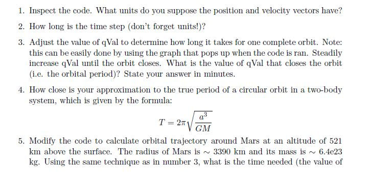
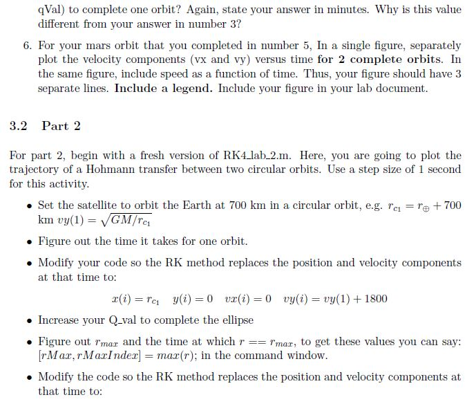
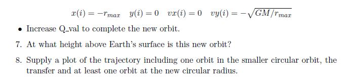
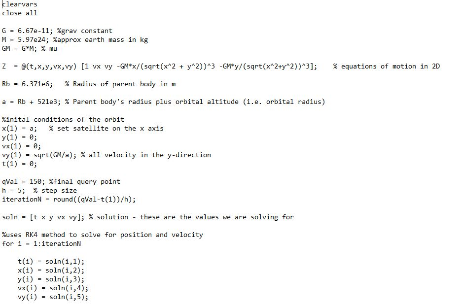
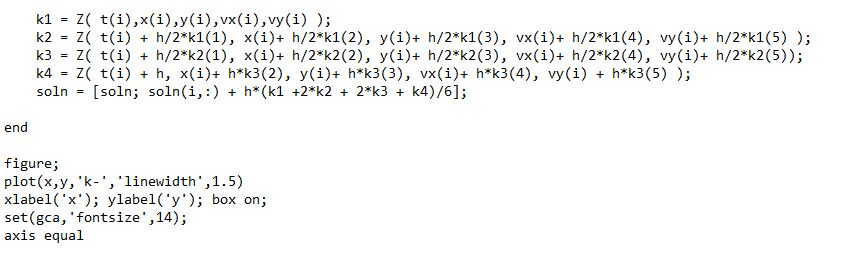
1. Inspect the code. What units do you suppose the position and velocity vectors have? 2. How long is the time step (don't forget units!)? 3. Adjust the value of Val to determine how long it takes for one complete orbit. Note: this can be easily done by using the graph that pops up when the code is ran. Steadily increase qVal until the orbit closes. What is the value of qval that closes the orbit (i.e. the orbital period)? State your answer in minutes. 4. How close is your approximation to the true period of a circular orbit in a two-body system, which is given by the formula: a T = 27V GM 5. Modify the code to calculate orbital trajectory around Mars at an altitude of 521 km above the surface. The radius of Mars is ~ 3390 km and its mass is ~ 6.4e23 kg. Using the same technique as in number 3, what is the time needed the value of qVal) to complete one orbit? Again, state your answer in minutes. Why is this value different from your answer in number 3? 6. For your mars orbit that you completed in number 5, In a single figure, separately plot the velocity components (vx and vy) versus time for 2 complete orbits. In the same figure, include speed as a function of time. Thus, your figure should have 3 separate lines. Include a legend. Include your figure in your lab document. 3.2 Part 2 For part 2, begin with a fresh version of RK4_lab_2.m. Here, you are going to plot the trajectory of a Hohmann transfer between two circular orbits. Use a step size of 1 second for this activity. Set the satellite to orbit the Earth at 700 km in a circular orbit, e.g. re=re + 700 km vy(1) = GM/re Figure out the time it takes for one orbit. Modify your code so the RK method replaces the position and velocity components at that time to: r(i) = rc y(i)=0 vr(i) = 0 vy(i) = vy(1) + 1800 Increase your Q_val to complete the ellipse . Figure out Imar and the time at which r == I'mar, to get these values you can say: [rMax, Maxinder] = max(r); in the command window. Modify the code so the RK method replaces the position and velocity components at that time to: r(i) = -r mar y(i)=0 vr(i) = 0 vy(i)=- GM /rmar Increase Q_val to complete the new orbit. 7. At what height above Earth's surface is this new orbit? 8. Supply a plot of the trajectory including one orbit in the smaller circular orbit, the transfer and at least one orbit at the new circular radius. clearvars close all G = 6.67e-11; %grav constant M = 5.97e24; %approx earth mass in kg GM = G*M; % mu % equations of motion in 2D Z = @(t,x,y,vx,vy) [1 vx vy -GM*x/(sqrt(x^2 + y^2))^3 -GM*y/(sqrt(x^2+y^2))^3]; Rb = 6.371e6; % Radius of parent body in m a = Rb + 521e3; % Parent body's radius plus orbital altitude (i.e. orbital radius) %inital conditions of the orbit x(1) = a; % set satellite on the x axis y(1) = 0; vx(1) = 0; vy(1) = sqrt(GM/a); % all velocity in the y-direction t(1) = 0; qVal - 150; %final query point h = 5; % step size iteration = round((Val-t(1))/h); soln = [t x y vx vy]; % solution - these are the values we are solving for %uses RK4 method to solve for position and velocity for i = 1:iterationN t(i) = soln(i,1); x(i) = soln(i, 2); y(i) = soln(i,3); vx(i) = soln(i, 4); vy(i) = soln(i,5); k1 = Z( t(i),x(i),y(i), vx(i), vy(i)); k2 = Z( t(i) + h/2*k1(1), x(i)+ h/2*k1(2), y(i)+ h/2*k1(3), vx(i)+ h/2*k1(4), vy(i)+ h/2*k1(5)); k3 = Z( t(i) + 1/2*k2(1), x(i)+ h/2*k2(2), y(i)+ h/2*k2(3), vx(i)+ h/2*k2(4), vy(i)+ h/2*k2(5)); k4 = Z( t(i) + h, x(i)+ h*k3(2), y(i)+ h*k3(3), vx(i)+ h*k3(4), vy(i) + h*k3(5) ); soln = (soln; soln(i,:) + h*(k1 +2*k2 + 2*k3 + k4)/6]; end figure; plot(x,y,'k-', 'linewidth',1.5) xlabel('x'); ylabel('y'); box on; set(gca,'fontsize',14); axis equal 1. Inspect the code. What units do you suppose the position and velocity vectors have? 2. How long is the time step (don't forget units!)? 3. Adjust the value of Val to determine how long it takes for one complete orbit. Note: this can be easily done by using the graph that pops up when the code is ran. Steadily increase qVal until the orbit closes. What is the value of qval that closes the orbit (i.e. the orbital period)? State your answer in minutes. 4. How close is your approximation to the true period of a circular orbit in a two-body system, which is given by the formula: a T = 27V GM 5. Modify the code to calculate orbital trajectory around Mars at an altitude of 521 km above the surface. The radius of Mars is ~ 3390 km and its mass is ~ 6.4e23 kg. Using the same technique as in number 3, what is the time needed the value of qVal) to complete one orbit? Again, state your answer in minutes. Why is this value different from your answer in number 3? 6. For your mars orbit that you completed in number 5, In a single figure, separately plot the velocity components (vx and vy) versus time for 2 complete orbits. In the same figure, include speed as a function of time. Thus, your figure should have 3 separate lines. Include a legend. Include your figure in your lab document. 3.2 Part 2 For part 2, begin with a fresh version of RK4_lab_2.m. Here, you are going to plot the trajectory of a Hohmann transfer between two circular orbits. Use a step size of 1 second for this activity. Set the satellite to orbit the Earth at 700 km in a circular orbit, e.g. re=re + 700 km vy(1) = GM/re Figure out the time it takes for one orbit. Modify your code so the RK method replaces the position and velocity components at that time to: r(i) = rc y(i)=0 vr(i) = 0 vy(i) = vy(1) + 1800 Increase your Q_val to complete the ellipse . Figure out Imar and the time at which r == I'mar, to get these values you can say: [rMax, Maxinder] = max(r); in the command window. Modify the code so the RK method replaces the position and velocity components at that time to: r(i) = -r mar y(i)=0 vr(i) = 0 vy(i)=- GM /rmar Increase Q_val to complete the new orbit. 7. At what height above Earth's surface is this new orbit? 8. Supply a plot of the trajectory including one orbit in the smaller circular orbit, the transfer and at least one orbit at the new circular radius. clearvars close all G = 6.67e-11; %grav constant M = 5.97e24; %approx earth mass in kg GM = G*M; % mu % equations of motion in 2D Z = @(t,x,y,vx,vy) [1 vx vy -GM*x/(sqrt(x^2 + y^2))^3 -GM*y/(sqrt(x^2+y^2))^3]; Rb = 6.371e6; % Radius of parent body in m a = Rb + 521e3; % Parent body's radius plus orbital altitude (i.e. orbital radius) %inital conditions of the orbit x(1) = a; % set satellite on the x axis y(1) = 0; vx(1) = 0; vy(1) = sqrt(GM/a); % all velocity in the y-direction t(1) = 0; qVal - 150; %final query point h = 5; % step size iteration = round((Val-t(1))/h); soln = [t x y vx vy]; % solution - these are the values we are solving for %uses RK4 method to solve for position and velocity for i = 1:iterationN t(i) = soln(i,1); x(i) = soln(i, 2); y(i) = soln(i,3); vx(i) = soln(i, 4); vy(i) = soln(i,5); k1 = Z( t(i),x(i),y(i), vx(i), vy(i)); k2 = Z( t(i) + h/2*k1(1), x(i)+ h/2*k1(2), y(i)+ h/2*k1(3), vx(i)+ h/2*k1(4), vy(i)+ h/2*k1(5)); k3 = Z( t(i) + 1/2*k2(1), x(i)+ h/2*k2(2), y(i)+ h/2*k2(3), vx(i)+ h/2*k2(4), vy(i)+ h/2*k2(5)); k4 = Z( t(i) + h, x(i)+ h*k3(2), y(i)+ h*k3(3), vx(i)+ h*k3(4), vy(i) + h*k3(5) ); soln = (soln; soln(i,:) + h*(k1 +2*k2 + 2*k3 + k4)/6]; end figure; plot(x,y,'k-', 'linewidth',1.5) xlabel('x'); ylabel('y'); box on; set(gca,'fontsize',14); axis equal