NEED ASAP!!!!

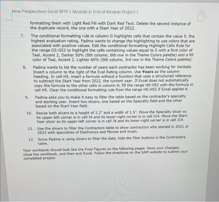
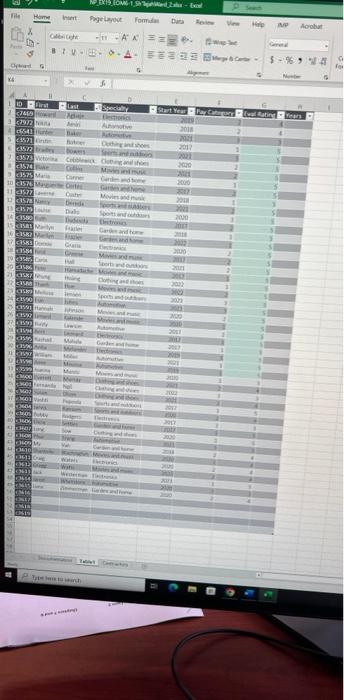
New Perspectives Excel 2019 | Module 6: End of Module Project 1 formatting them with Light Red Fill with Dark Red Text. Delete the second instance of the duplicate record, the one with a Start Year of 2022. 7. The conditional formatting rule in column G highlights cells that contain the value 5 , the highest evaluation rating. Padma wants to change the highlighting to use colors that are associated with positive values. Edit the conditional formatting Highlight Cells Rule for the range G5:G52 to highlight the cells containing values equal to 5 with a font color of Teal, Accent 2, Darker 50% (6th column, 6th row in the Theme Colors palette) and a fill color of Teal, Accent 2, Lighter 60% (6th column, 3rd row in the Theme Colors palette). 8. Padma wants to list the number of years each contractor has been working for Veritate. Insert a column to the right of the Eval Rating column. Use Years as the column heading. In cell H5, insert a formula without a function that uses a structured reference to subtract the Start Year from 2022, the current year. If Excel does not automatically copy the formula to the other cells in column H, fill the range H6:H52 with the formula in cell H5. Clear the conditional formatting rule from the range H5:H52 if Excel applies it. 9. Padma asks you to make it easy to filter the table based on the contractor's specialty and starting year. Insert two slicers, one based on the Specialty field and the other based on the Start Year field. 10. Resize both slicers to a height of 2.2 and a width of 1.5. Move the Specialty slicer so its upper-left corner is in cell 14 and its lower-right corner is in cell I14. Move the Start Year slicer so its upper-left comer is in cell J4 and its lower-right corner is in cell J14. 11. Use the slicers to filter the Contractors table to show contractors who started in 2021 or 2022 with specialties of Electronics and Movies and music. 12. Since Padma is using slicers to filter the data, hide the filter buttons in the Contractors table. Your workbook should look like the Final Figures on the following pages. Save your changes, close the workbook, and then exit Excel. Follow the directions on the SAM website to submit your completed project. New Perspectives Excel 2019 | Module 6: End of Module Project 1 formatting them with Light Red Fill with Dark Red Text. Delete the second instance of the duplicate record, the one with a Start Year of 2022. 7. The conditional formatting rule in column G highlights cells that contain the value 5 , the highest evaluation rating. Padma wants to change the highlighting to use colors that are associated with positive values. Edit the conditional formatting Highlight Cells Rule for the range G5:G52 to highlight the cells containing values equal to 5 with a font color of Teal, Accent 2, Darker 50% (6th column, 6th row in the Theme Colors palette) and a fill color of Teal, Accent 2, Lighter 60% (6th column, 3rd row in the Theme Colors palette). 8. Padma wants to list the number of years each contractor has been working for Veritate. Insert a column to the right of the Eval Rating column. Use Years as the column heading. In cell H5, insert a formula without a function that uses a structured reference to subtract the Start Year from 2022, the current year. If Excel does not automatically copy the formula to the other cells in column H, fill the range H6:H52 with the formula in cell H5. Clear the conditional formatting rule from the range H5:H52 if Excel applies it. 9. Padma asks you to make it easy to filter the table based on the contractor's specialty and starting year. Insert two slicers, one based on the Specialty field and the other based on the Start Year field. 10. Resize both slicers to a height of 2.2 and a width of 1.5. Move the Specialty slicer so its upper-left corner is in cell 14 and its lower-right corner is in cell I14. Move the Start Year slicer so its upper-left comer is in cell J4 and its lower-right corner is in cell J14. 11. Use the slicers to filter the Contractors table to show contractors who started in 2021 or 2022 with specialties of Electronics and Movies and music. 12. Since Padma is using slicers to filter the data, hide the filter buttons in the Contractors table. Your workbook should look like the Final Figures on the following pages. Save your changes, close the workbook, and then exit Excel. Follow the directions on the SAM website to submit your completed project