NEED HELP BADLY PLEASE THANKS ANY HELP IS APPRECIATED. CODING IS DONE IN MATLAB

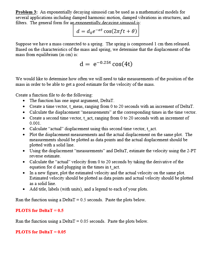
Problem 3: An exponentially decaying sinusoid can be used as a mathematical models for several applications including damped harmonic motion, damped vibrations in structures, and filters. The general form for Suppose we have a mass connected to a spring. The spring is compressed 1 cm then released Based on the characteristics of the mass and spring, we determine that the displacement of the mass from equilibrium (in cm) is e-0.25t cos(4t) = We would like to determine how often we will need to take measurements of the position of the mass in order to be able to get a good estimate for the velocity of the mas:s Create a function file to do the following . The function has one input argument, DeltaT . Create a time vector, t meas, ranging from 0 to 20 seconds with an increment of DeltaT . Calculate the displacement "measurements" at the corresponding times in the time vector .Create a second time vector, t act, ranging from 0 to 20 seconds with an increment of 0.001 . Calculate "actual" displacement using this second time vector, t_act. .Plot the displacement measurements and the actual displacement on the same plot. The measurements should be plotted as data points and the actual displacement should be plotted with a solid line Using the displacement "measurements" and DeltaT, estimate the velocity using the 2-PT reverse estimate Calculate the "actual" velocity from 0 to 20 seconds by taking the derivative of the equation for d and plugging in the times in t_act. . . In a new figure, plot the estimated velocity and the actual velocity on the same plot. Estimated velocity should be plotted as data points and actual velocity should be plotted as a solid line .Add title, labels (with units), and a legend to each of your plots. Run the function using a DeltaT = 0.5 seconds. Paste the plots below PLOTS for DeltaT 0.5 Run the function using a DeltaT = 0.05 seconds. Paste the plots below PLOTS for DeltaT 0.05 Problem 3: An exponentially decaying sinusoid can be used as a mathematical models for several applications including damped harmonic motion, damped vibrations in structures, and filters. The general form for Suppose we have a mass connected to a spring. The spring is compressed 1 cm then released Based on the characteristics of the mass and spring, we determine that the displacement of the mass from equilibrium (in cm) is e-0.25t cos(4t) = We would like to determine how often we will need to take measurements of the position of the mass in order to be able to get a good estimate for the velocity of the mas:s Create a function file to do the following . The function has one input argument, DeltaT . Create a time vector, t meas, ranging from 0 to 20 seconds with an increment of DeltaT . Calculate the displacement "measurements" at the corresponding times in the time vector .Create a second time vector, t act, ranging from 0 to 20 seconds with an increment of 0.001 . Calculate "actual" displacement using this second time vector, t_act. .Plot the displacement measurements and the actual displacement on the same plot. The measurements should be plotted as data points and the actual displacement should be plotted with a solid line Using the displacement "measurements" and DeltaT, estimate the velocity using the 2-PT reverse estimate Calculate the "actual" velocity from 0 to 20 seconds by taking the derivative of the equation for d and plugging in the times in t_act. . . In a new figure, plot the estimated velocity and the actual velocity on the same plot. Estimated velocity should be plotted as data points and actual velocity should be plotted as a solid line .Add title, labels (with units), and a legend to each of your plots. Run the function using a DeltaT = 0.5 seconds. Paste the plots below PLOTS for DeltaT 0.5 Run the function using a DeltaT = 0.05 seconds. Paste the plots below PLOTS for DeltaT 0.05