Answered step by step
Verified Expert Solution
Question
1 Approved Answer
NEED HELP WITH SAM PROJECT!! GETTING STARTED - Open the file NP_EX19_7a_FirstLastName_1.xisx, avallable for download from the SAM website. - Save the file as NP_EX19_7a_FirstLastName_2.xisx
NEED HELP WITH SAM PROJECT!! 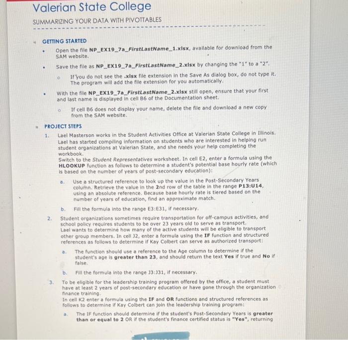

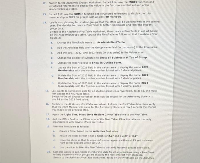
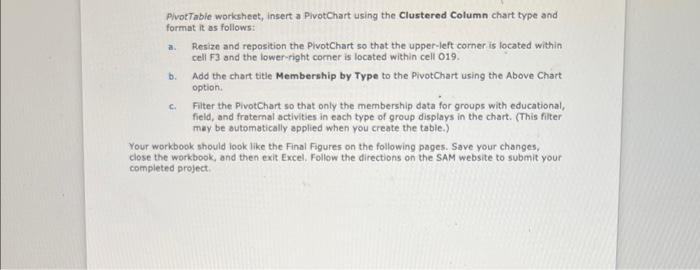
GETTING STARTED - Open the file NP_EX19_7a_FirstLastName_1.xisx, avallable for download from the SAM website. - Save the file as NP_EX19_7a_FirstLastName_2.xisx by changing the "1" to a " 2 ". If you do not see the -xisx file extension in the Save As dialog box, do not type it. The program will add the file extension for you automatically. - With the file NP_EX19_7a_FirstLastName_2.xisx still open, ensure that your first and last name is displayed in cell B6 of the Documentation sheet. If cell B6 does not display your name, delete the file and download a new copy from the SAM website. PROJECT STEPS 1. Lael Masterson works in the Student Activities Office at Valerian State College in tillinois. Lael has started compiling information on students who are interested in helping run student organizations at Valerian State, and she needs your help completing the workbook. Switch to the Student Representatives worksheet, In cell E2, enter a formula using the HLOOKUP function as follows to determine a student's potential base hourly rate (which is based on the number of years of post-secondary education): a. Use a structured reference to look up the value in the Post-Secondary Years column. Retrieve the value in the 2 nd row of the table in the range P13:U14, using an absolute reference. Because base hourly rate is tiered based on the number of years of education, find an approximate match. b. Fill the formula into the range E3:E31, if necessary. 2. Student organizations sometimes require transportation for off-campus activities, and school policy requires students to be over 23 years old to serve as transport. Lael wants to determine how many of the active students will be eligible to transport other group members. In cell 32 , enter a formula using the IF function and structured references as follows to determine if Kay Colbert can serve as authorized transport: a. The function should use a reference to the Age column to determine if the student's age is greater than 23 , and should return the text Yes if true and No if false. b. Fill the formula into the range 33:331, if necessary. 3. To be eligible for the leadership training program offered by the office, a student must have at least 2 years of post-secondary education or have gone through the organization finance training. In cell K2 enter a formula using the IF and OR functions and structured references as follows to determine if Kay Colbert can join the leadership training program: a. The IF function should determine if the student's Post-Secondary Years is greater than or equal to 2 OR if the student's finance certified status is "Yes", returning the text Yes if a student meets one or both of those criteria or the text No if a student meets neither of those criteria. b. Fill the formula into the range K3:K31, If necessary. 4. Experienced students may serve as mentors if they are at least age 21 and have at least 3 years of post-secondary education. In cell LZ, enter a formula using the If and AND functions and structured references as follows to determine if Kay Colbert is eligible to serve as a mentor: a. The IF function should determine if the student's age is greater than or equal to 21 AND the student's post-secondary years are greater than or equal to 3 , and should return the text Yes if a student meets both of those criteria or the text No if a student meets none of only one of those criteria. b. Fill the formula into the range L3:L.31, if necessary. 5. Lael is always on the lookout for students who might be interested in running for office in student groups. In cell M2, enter a formula using a nested If function and structured references as follows to determine first if a student has already been elected to office in a student group, and if not, whether that student meets the qualifications to run in the future: a. If the value in the Elected column is equal to the text "Yes", the formula should display Elected as the text. b. Otherwise, the formula should determine if the value in the Finance Certified column is equal to the text "Yes" and return the text Yes if true And No if false. 6. Students who work with student organizations are also considered for employment at the Student Activities Office. Students with more than 4 years of post-secondary education are qualified for more complex Tier 2 jobs. In cell N1, enter the text Tier as the column heading. 7. In cell N2, enter a formula using the IF function and structured references as follows to determine which work tier Kay Colbert is qualified for: a. The If function should determine if the student's Post-Secondary Years is greater than or equal to 4 , and return the value 2 if true or the value 1 if false. b. Fill the formula into the range N3:N31, if necessary. 8. Lael wants a quick way to look up students by their 5 tudent ID. In cell Q3, hest the existing VLOOKUP function in an XFERROR function. If the VLOOKUP function retums an error result, the text Invalid Student ID should display. 9. Lael wants to determine several totais and averages for active students: In cell Q8, enter a formula using the COUNTIF function and structured references to count the number of students who have been elected to offices in student organizations. 10. In cell R.b, enter oformula using the AVERAGEIF function and structured references to determine the average number of post-secondary vears for students who have been elected. 11. In cell R9, enter a formula using the AvRRAGE function and structured references to determine the average number of years of post-secondary education of all students as shown in the Post-Secondary Years column. 12. Switch to the Academic Groups worksheet. In cell A14, use the INDEX function and structured references to display the value in the first row and first column of the AcademicGroups table. 13. In cell A17, use the SUMIF function and structured references to display the total membership in 2023 for groups with ot least 40 members. 14. Lael is also planning for student groups that the office will be working with in the coming year. She decides to create a PivotTable to better manipulate and filter the student. group data. Switch to the Academic PivorTable worksheet, then create a PivotTable in cell A1 based on the AcodemicGroups table. Update the PivotTable as follows so that it matches Final Figure 2: a. Change the PivotTable name to: AcademicPivotTable b. Add the Activities field and the Group Name field (in that order) to the Rows area. c. Add the 2021, 2022, and 2023 fields (in that order) to the Values area. d. Change the display of subtotals to Show all Subtotals at Top of Group. e. Change the report layout to Show in Outline Form. t. Update the Sum of 2021 field in the Values area to display the name 2021 Membership with the Number number format with 0 decimal places. 9. Update the Sum of 2022 field in the Values area to display the name 2022 Membership with the Number number format with 0 decimat places. h. Update the 5 um of 2023 field in the Values area to display the name 2023 Membership with the Number number format with 0 decimal places. 15. Lael wants to summarite data for ali student graups in a PivotTable. To do so, she must frit update the AliGroups table. Switch to the All Groups worksheet then edit the record for the Astronomy Society to use 76 as the 2023 field value. 16. Switch to the Ali Groups AvotTable worksheet. Refresh the PivotTable data, theen verify that the 2023 Membership value for the Astronomy Society in row 6 reflects the change You made in the previous step. 17. Apply the Light Blue, Pivot style Medium 2 PivotTable style to the PivotTabie. 18. Add the Olfice field to the Filters area of the Pivot Table. Filter the table so that only organizations with private offices are visibie. 19. Fiter the PivotTable as follows: a. Create a sticer based on the Activities fieid value. b. Hevize the slicer so that it has a height of 2.2 and a width of 3.2. c. Move the slicer so that its upper-left comer appears within cell Fis and its lowee-: right comer appears within cell 314 . d. Use the slicer to fiter the PivotTable so that only Fraternal groups are visible. 20. Lael also wants to summarize membership data for all organizations using a pivetchart: to help determine which groups are showing the most interest from students. Switch to the Activities PivotTable worksheet, Based on then Pivotrabie on the Activities PivotTable worksheet, insert a PivotChart using the Clustered Column chart type and format it as follows: a. Resize and reposition the PivotChart so that the upper-left corner is located within cell F3 and the lower-right comer is located within cell 019 . b. Add the chart title Membership by Type to the PivotChart using the Above Chart option. c. Filter the PivotChart so that only the membership data for groups with educational, field, and fratemal activities in each type of group displays in the chart. (This filter may be automatically applied when you create the tabie.) or workbook should look like the Final Figures on the following pages. Save your changes, se the workbook, and then exit Excel. Follow the directions on the SAM website to submit your npleted project. GETTING STARTED - Open the file NP_EX19_7a_FirstLastName_1.xisx, avallable for download from the SAM website. - Save the file as NP_EX19_7a_FirstLastName_2.xisx by changing the "1" to a " 2 ". If you do not see the -xisx file extension in the Save As dialog box, do not type it. The program will add the file extension for you automatically. - With the file NP_EX19_7a_FirstLastName_2.xisx still open, ensure that your first and last name is displayed in cell B6 of the Documentation sheet. If cell B6 does not display your name, delete the file and download a new copy from the SAM website. PROJECT STEPS 1. Lael Masterson works in the Student Activities Office at Valerian State College in tillinois. Lael has started compiling information on students who are interested in helping run student organizations at Valerian State, and she needs your help completing the workbook. Switch to the Student Representatives worksheet, In cell E2, enter a formula using the HLOOKUP function as follows to determine a student's potential base hourly rate (which is based on the number of years of post-secondary education): a. Use a structured reference to look up the value in the Post-Secondary Years column. Retrieve the value in the 2 nd row of the table in the range P13:U14, using an absolute reference. Because base hourly rate is tiered based on the number of years of education, find an approximate match. b. Fill the formula into the range E3:E31, if necessary. 2. Student organizations sometimes require transportation for off-campus activities, and school policy requires students to be over 23 years old to serve as transport. Lael wants to determine how many of the active students will be eligible to transport other group members. In cell 32 , enter a formula using the IF function and structured references as follows to determine if Kay Colbert can serve as authorized transport: a. The function should use a reference to the Age column to determine if the student's age is greater than 23 , and should return the text Yes if true and No if false. b. Fill the formula into the range 33:331, if necessary. 3. To be eligible for the leadership training program offered by the office, a student must have at least 2 years of post-secondary education or have gone through the organization finance training. In cell K2 enter a formula using the IF and OR functions and structured references as follows to determine if Kay Colbert can join the leadership training program: a. The IF function should determine if the student's Post-Secondary Years is greater than or equal to 2 OR if the student's finance certified status is "Yes", returning the text Yes if a student meets one or both of those criteria or the text No if a student meets neither of those criteria. b. Fill the formula into the range K3:K31, If necessary. 4. Experienced students may serve as mentors if they are at least age 21 and have at least 3 years of post-secondary education. In cell LZ, enter a formula using the If and AND functions and structured references as follows to determine if Kay Colbert is eligible to serve as a mentor: a. The IF function should determine if the student's age is greater than or equal to 21 AND the student's post-secondary years are greater than or equal to 3 , and should return the text Yes if a student meets both of those criteria or the text No if a student meets none of only one of those criteria. b. Fill the formula into the range L3:L.31, if necessary. 5. Lael is always on the lookout for students who might be interested in running for office in student groups. In cell M2, enter a formula using a nested If function and structured references as follows to determine first if a student has already been elected to office in a student group, and if not, whether that student meets the qualifications to run in the future: a. If the value in the Elected column is equal to the text "Yes", the formula should display Elected as the text. b. Otherwise, the formula should determine if the value in the Finance Certified column is equal to the text "Yes" and return the text Yes if true And No if false. 6. Students who work with student organizations are also considered for employment at the Student Activities Office. Students with more than 4 years of post-secondary education are qualified for more complex Tier 2 jobs. In cell N1, enter the text Tier as the column heading. 7. In cell N2, enter a formula using the IF function and structured references as follows to determine which work tier Kay Colbert is qualified for: a. The If function should determine if the student's Post-Secondary Years is greater than or equal to 4 , and return the value 2 if true or the value 1 if false. b. Fill the formula into the range N3:N31, if necessary. 8. Lael wants a quick way to look up students by their 5 tudent ID. In cell Q3, hest the existing VLOOKUP function in an XFERROR function. If the VLOOKUP function retums an error result, the text Invalid Student ID should display. 9. Lael wants to determine several totais and averages for active students: In cell Q8, enter a formula using the COUNTIF function and structured references to count the number of students who have been elected to offices in student organizations. 10. In cell R.b, enter oformula using the AVERAGEIF function and structured references to determine the average number of post-secondary vears for students who have been elected. 11. In cell R9, enter a formula using the AvRRAGE function and structured references to determine the average number of years of post-secondary education of all students as shown in the Post-Secondary Years column. 12. Switch to the Academic Groups worksheet. In cell A14, use the INDEX function and structured references to display the value in the first row and first column of the AcademicGroups table. 13. In cell A17, use the SUMIF function and structured references to display the total membership in 2023 for groups with ot least 40 members. 14. Lael is also planning for student groups that the office will be working with in the coming year. She decides to create a PivotTable to better manipulate and filter the student. group data. Switch to the Academic PivorTable worksheet, then create a PivotTable in cell A1 based on the AcodemicGroups table. Update the PivotTable as follows so that it matches Final Figure 2: a. Change the PivotTable name to: AcademicPivotTable b. Add the Activities field and the Group Name field (in that order) to the Rows area. c. Add the 2021, 2022, and 2023 fields (in that order) to the Values area. d. Change the display of subtotals to Show all Subtotals at Top of Group. e. Change the report layout to Show in Outline Form. t. Update the Sum of 2021 field in the Values area to display the name 2021 Membership with the Number number format with 0 decimal places. 9. Update the Sum of 2022 field in the Values area to display the name 2022 Membership with the Number number format with 0 decimat places. h. Update the 5 um of 2023 field in the Values area to display the name 2023 Membership with the Number number format with 0 decimal places. 15. Lael wants to summarite data for ali student graups in a PivotTable. To do so, she must frit update the AliGroups table. Switch to the All Groups worksheet then edit the record for the Astronomy Society to use 76 as the 2023 field value. 16. Switch to the Ali Groups AvotTable worksheet. Refresh the PivotTable data, theen verify that the 2023 Membership value for the Astronomy Society in row 6 reflects the change You made in the previous step. 17. Apply the Light Blue, Pivot style Medium 2 PivotTable style to the PivotTabie. 18. Add the Olfice field to the Filters area of the Pivot Table. Filter the table so that only organizations with private offices are visibie. 19. Fiter the PivotTable as follows: a. Create a sticer based on the Activities fieid value. b. Hevize the slicer so that it has a height of 2.2 and a width of 3.2. c. Move the slicer so that its upper-left comer appears within cell Fis and its lowee-: right comer appears within cell 314 . d. Use the slicer to fiter the PivotTable so that only Fraternal groups are visible. 20. Lael also wants to summarize membership data for all organizations using a pivetchart: to help determine which groups are showing the most interest from students. Switch to the Activities PivotTable worksheet, Based on then Pivotrabie on the Activities PivotTable worksheet, insert a PivotChart using the Clustered Column chart type and format it as follows: a. Resize and reposition the PivotChart so that the upper-left corner is located within cell F3 and the lower-right comer is located within cell 019 . b. Add the chart title Membership by Type to the PivotChart using the Above Chart option. c. Filter the PivotChart so that only the membership data for groups with educational, field, and fratemal activities in each type of group displays in the chart. (This filter may be automatically applied when you create the tabie.) or workbook should look like the Final Figures on the following pages. Save your changes, se the workbook, and then exit Excel. Follow the directions on the SAM website to submit your npleted project 


Step by Step Solution
There are 3 Steps involved in it
Step: 1

Get Instant Access to Expert-Tailored Solutions
See step-by-step solutions with expert insights and AI powered tools for academic success
Step: 2

Step: 3

Ace Your Homework with AI
Get the answers you need in no time with our AI-driven, step-by-step assistance
Get Started


