Need help with screenshots 6, 7, 8, 9, and 10. Note: screenshot 7 has two screenshots, as it would not fit in one screenshot. So, whenever you scroll down and see a blank screenshot, know that it is "part 2" of "screenshot 7, part 1." Let me know if you need any more info!!

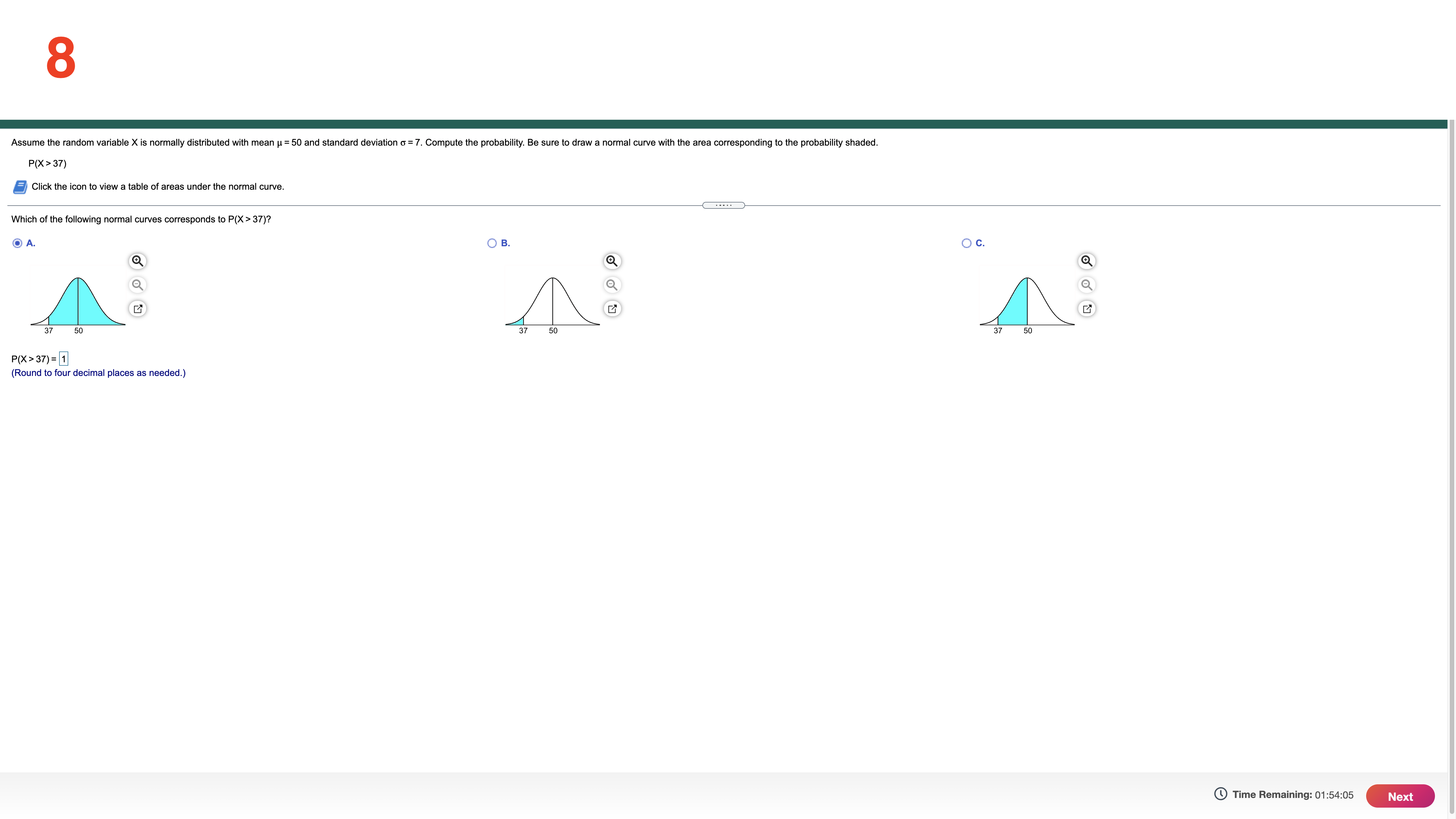
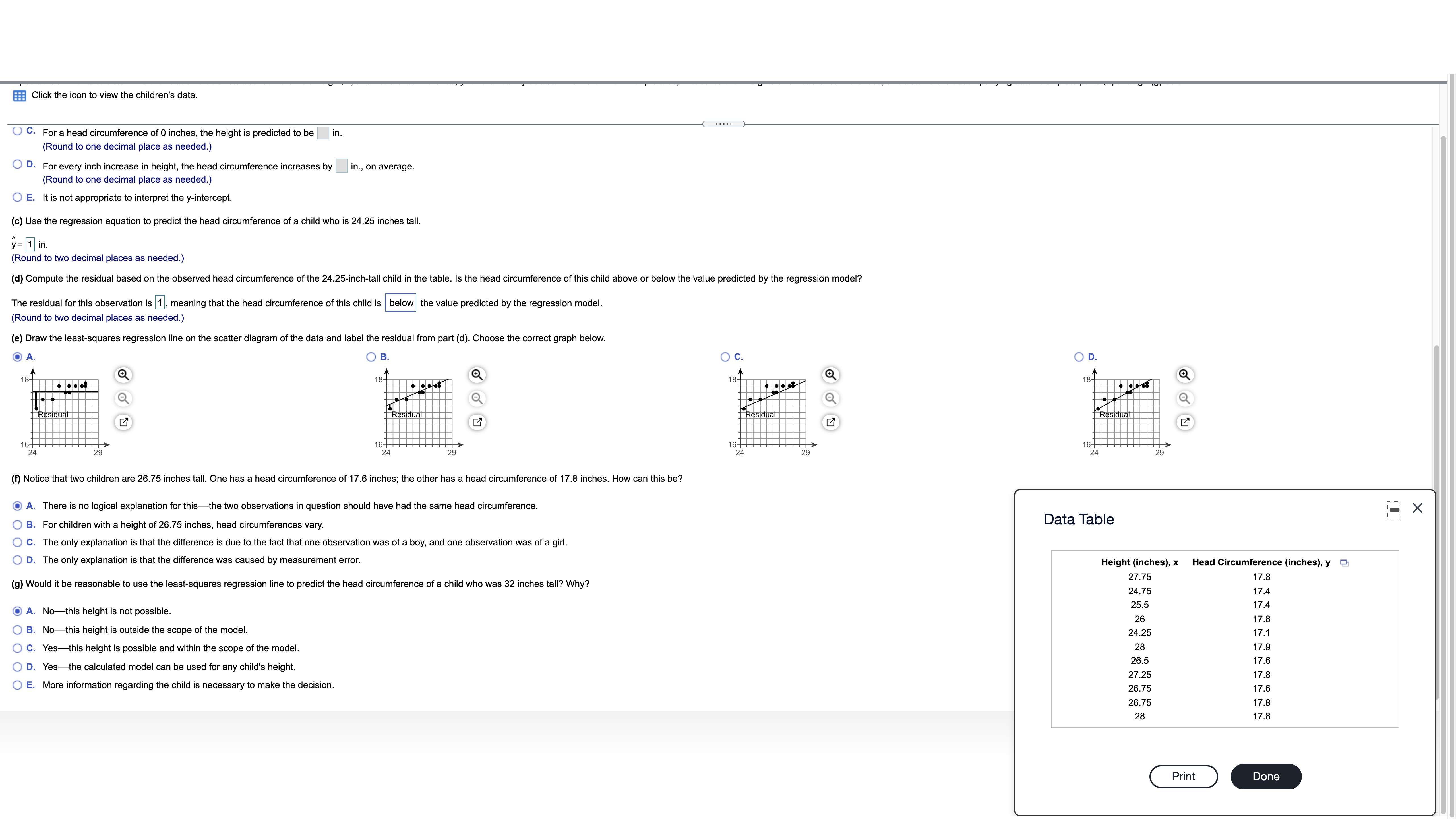
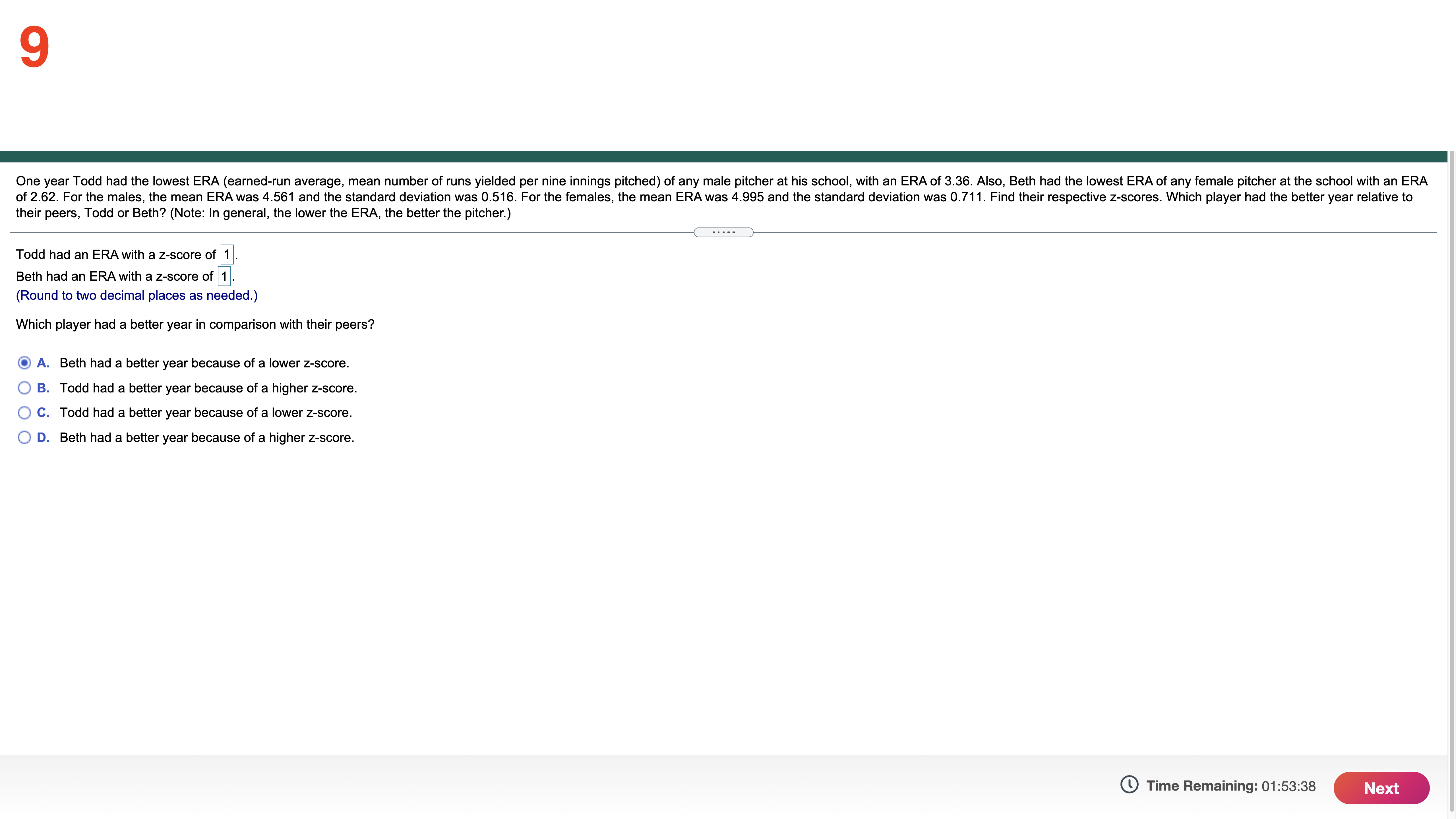
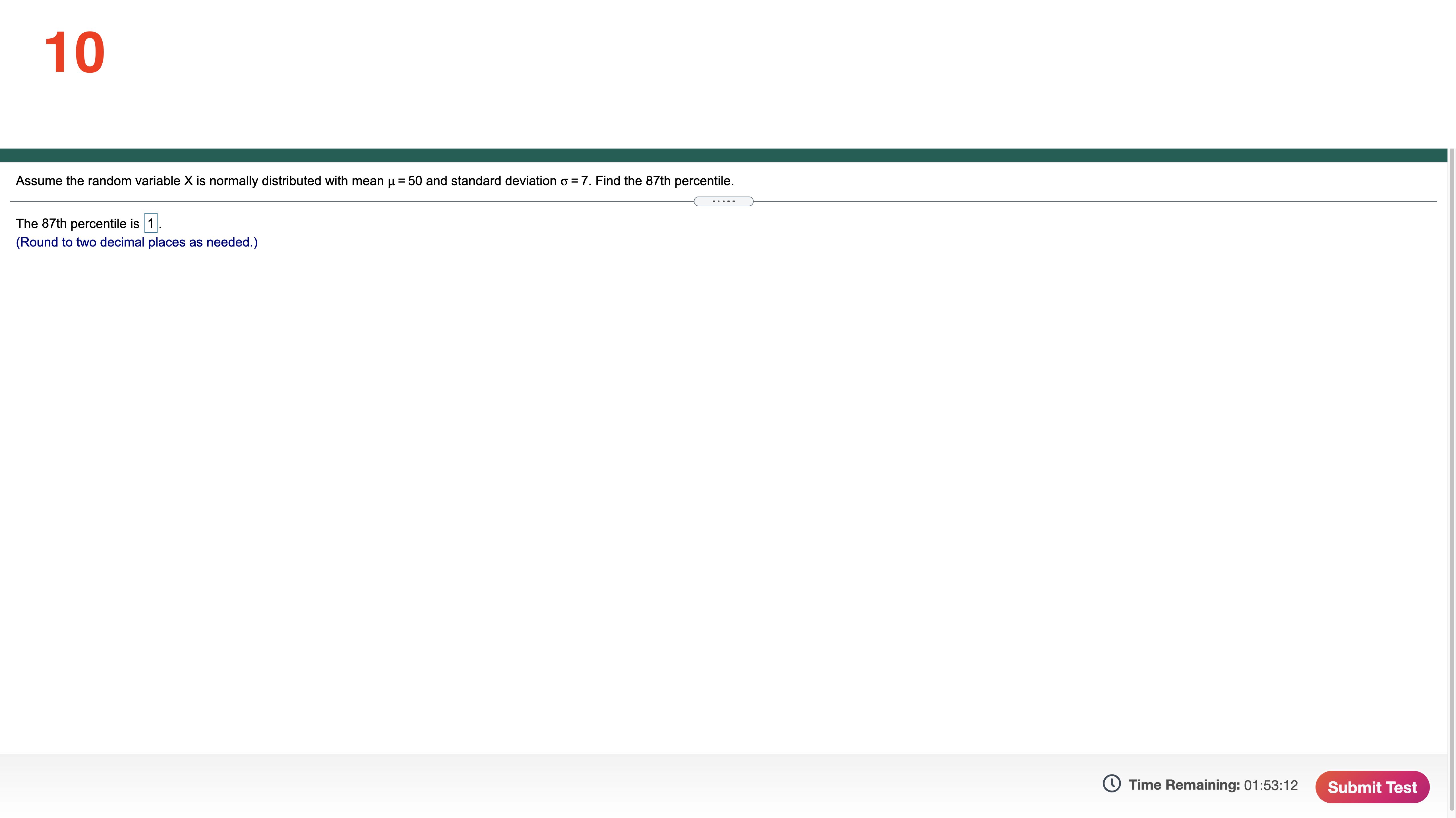
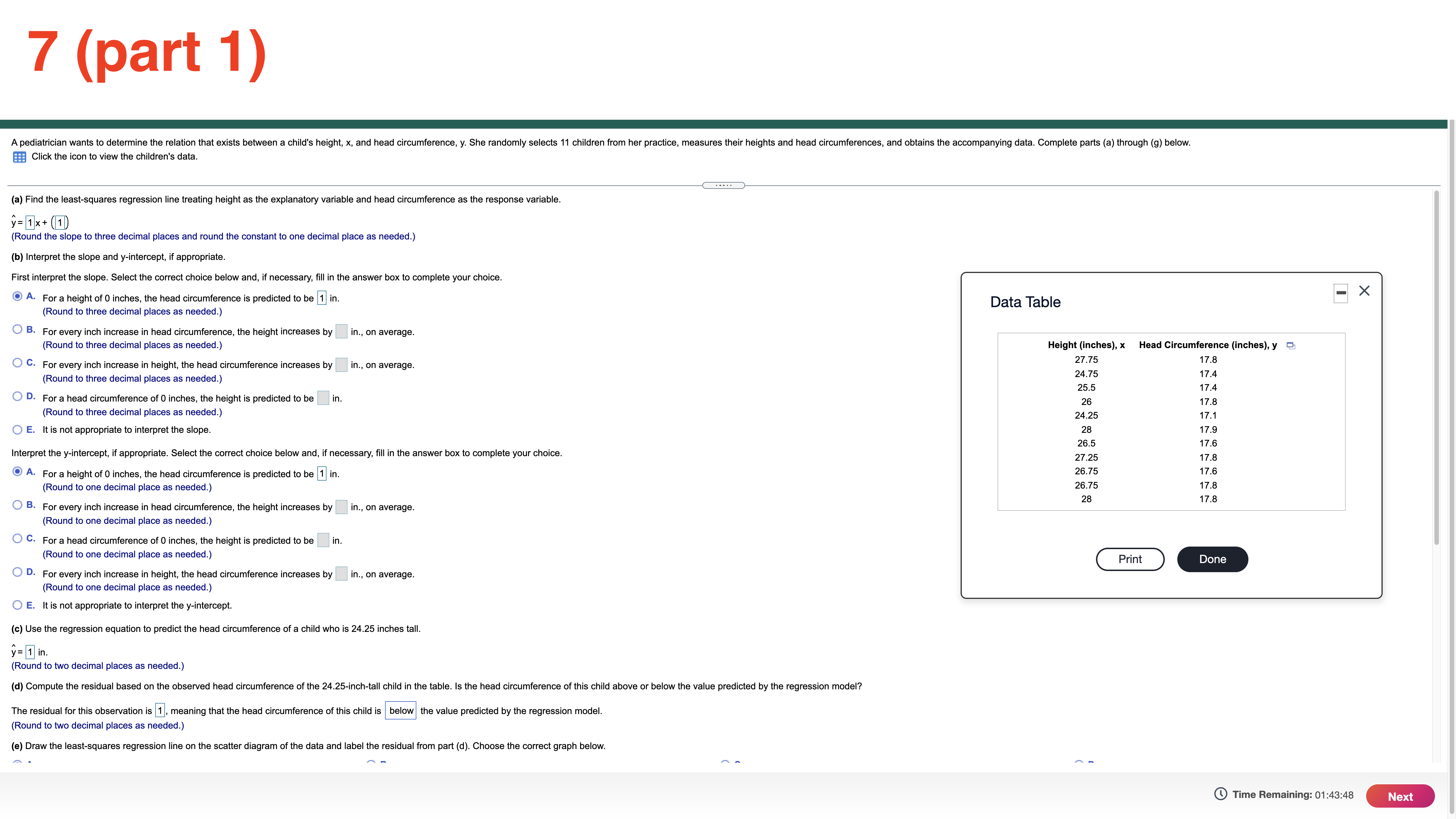
6 Suppose that E and F are two events and that N(E and F) = 370 and N(E) = 850. What is P(FIE)? P(FIE) ~ 1 (Round to three decimal places as needed.) Time Remaining: 01:55:32 Next8 Assume the random variable X is normally distributed with mean u = 50 and standard deviation o = 7. Compute the probability. Be sure to draw a normal curve with the area corresponding to the probability shaded. P(X > 37) Click the icon to view a table of areas under the normal curve. Which of the following normal curves corresponds to P(X > 37)? A O B OC 37 50 37 50 37 50 P(X > 37) = 1 (Round to four decimal places as needed.) Time Remaining: 01:54:05 Next9 One year Todd had the lowest ERA (earned-run average, mean number of runs yielded per nine innings pitched) of any male pitcher at his school, with an ERA of 3.36. Also, Beth had the lowest ERA of any female pitcher at the school with an ERA of 2.62. For the males, the mean ERA was 4.561 and the standard deviation was 0.516. For the females, the mean ERA was 4.995 and the standard deviation was 0.711. Find their respective z-soores. Which player had the better year relative to their peers, Todd or Beth? (Note: In general, the lower the ERA, the better the pitcher.) Todd had an ERA with a zscore of 1 . Beth had an ERA with a z-soore of 1 . (Round to two decimal places as needed.) Which player had a better year in comparison with their peers? A. Beth had a better year because of a lower z-soore. O B. Todd had a better year because of a higher z-score. O 0. Todd had a better year because of a lower z-score. O D. Beth had a better year because of a higher z-soore. Time Remaining: 01:53:38 m 10 Assume the random variable X is normally distributed with mean p= 50 and standard deviation 0 = 7. Find the 87th percentile The 87th percentile is 1 . (Round to two decimal places as needed.) Time Remaining: 01:53:12 Submit Test 7 (part 1) A pediatrician wants to determine the relation that exists between a child's height, x, and head circumference, y. She randomly selects 11 children from her practice, measures their heights and head circumferences, and obtains the accompanying data. Complete parts (a) through (9) below. Click the icon to view the children's data. (a) Find the least-squares regression line treating height as the explanatory variable and head circumference as the response variable. y = 1x + 1 (Round the slope to three decimal places and round the constant to one decimal place as needed.) (b) Interpret the slope and y-intercept, if appropriate. First interpret the slope. Select the correct choice below and, if necessary, fill in the answer box to complete your choice. A. For a height of 0 inches, the head circumference is predicted to be 1 in. -X Data Table (Round to three decimal places as needed.) O B. For every inch increase in head circumference, the height increases by |in., on average (Round to three decimal places as needed.) Height (inches), x Head Circumference (inches), y C. For every inch increase in height, the head circumference increases by |in., on average. 27.75 17. Round to three decimal places as needed.) 24.75 17.4 25.5 17.4 O D. For a head circumference of 0 inches, the height is predicted to be |in. 26 17.8 Round to three decimal places as needed.) 24.25 7.1 O E. It is not appropriate to interpret the slope. 28 17.9 26.5 17.6 Interpret the y-intercept, if appropriate. Select the correct choice below and, if necessary, fill in the answer box to complete your choice. 27.25 17.8 O A. For a height of 0 inches, the head circumference is predicted to be 1 in. 26.75 7.6 (Round to one decimal place as needed.) 26.75 17.8 28 17.8 O B. For every inch increase in head circumference, the height increases by in., on average. (Round to one decimal place as needed.) O C. For a head circumference of 0 inches, the height is predicted to be |in. (Round to one decimal place as needed.) Print Done O D. For every inch increase in height, the head circumference increases by in., on average. Round to one decimal place as needed. O E. It is not appropriate to interpret the y-intercept. (c) Use the regression equation to predict the head circumference of a child who is 24.25 inches tall. y= 1 in. (Round to two decimal places as needed.) (d) Compute the residual based on the observed head circumference of the 24.25-inch-tall child in the table. Is the head circumference of this child above or below the value predicted by the regression model? The residual for this observation is 1 , meaning that the head circumference of this child is below the value predicted by the regression model. (Round to two decimal places as needed.) (e) Draw the least-squares regression line on the scatter diagram of the data and label the residual from part (d). Choose the correct graph below. Time Remaining: 01:43:48 NextClick the icon to view the children's data. O C. For a head circumference of 0 inches, the height is predicted to be in. (Round to one decimal place as needed.) O D. For every inch increase in height, the head circumference increases by in., on average. Round to one decimal place as needed.) O E. It is not appropriate to interpret the y-intercept. (c) Use the regression equation to predict the head circumference of a child who is 24.25 inches tall. y = 1 in . (Round to two decimal places as needed.) (d) Compute the residual based on the observed head circumference of the 24.25-inch-tall child in the table. Is the head circumference of this child above or below the value predicted by the regression model? The residual for this observation is 1, meaning that the head circumference of this child is |below the value predicted by the regression model. (Round to two decimal places as needed.) (e) Draw the least-squares regression line on the scatter diagram of the data and label the residual from part (d). Choose the correct graph below. OA O B. O c. O D. 18- 18- Q 18 7 1 R Residual 6- (f) Notice that two children are 26.75 inches tall. One has a head circumference of 17.6 inches; the other has a head circumference of 17.8 inches. How can this be? O A. There is no logical explanation for this-the two observations in question should have had the same head circumference. -X O B. For children with a height of 26.75 inches, head circumferences vary Data Table O C. The only explanation is that the difference is due to the fact that one observation was of a boy, and one observation was of a girl. O D. The only explanation is that the difference was caused by measurement error. Height (inches), x Head Circumference (inches), y 27.75 17.8 g) Would it be reasonable to use the least-squares regression line to predict the head circumference of a child who was 32 inches tall? Why? 24.75 17.4 O A. No-this height is not possible. 25.5 17.4 26 17.8 O B. No-this height is outside the scope of the model 24.25 17.1 O C. Yes-this height is possible and within the scope of the model. 28 17.9 O D. Yes-the calculated model can be used for any child's height. 26.5 17.6 27.25 17.8 O E. More information regarding the child is necessary to make the decision. 26.75 17.6 26.75 17.8 28 17.8 Print Done