Need solution and explanation (code in the function given)
cannot use stuff like numpy or pandas
def greedy_predictor(data, y): """ This implements a greedy correlation pursuit algorithm. >>> data = [[1, 0], ... [2, 3], ... [4, 2]] >>> y = [2, 1, 2] >>> weights, intercept = greedy_predictor(data, y) >>> round(weights[0],2) 0.21 >>> round(weights[1],2) -0.29 >>> round(intercept, 2) 1.64 >>> data = [[0, 0], ... [1, 0], ... [0, -1]] >>> y = [1, 0, 0] >>> weights, intercept = greedy_predictor(data, y) >>> round(weights[0],2) -0.5 >>> round(weights[1],2) 0.75 >>> round(intercept, 2) 0.75 """ passdef equation(i, data, y): """ Finds the row representation of the i-th least squares condition, i.e., the equation representing the orthogonality of the residual on data column i: (x_i)'(y-Xb) = 0 (x_i)'Xb = (x_i)'y x_(1,i)*[x_11, x_12,..., x_1n] + ... + x_(m,i)*[x_m1, x_m2,..., x_mn] = For example: >>> data = [[1, 0], ... [2, 3], ... [4, 2]] >>> y = [2, 1, 2] >>> coeffs, rhs = equation(0, data, y) >>> round(coeffs[0],2) 4.67 >>> round(coeffs[1],2) 2.33 >>> round(rhs,2) 0.33 >>> coeffs, rhs = equation(1, data, y) >>> round(coeffs[0],2) 2.33 >>> round(coeffs[1],2) 4.67 >>> round(rhs,2) -1.33 """ passdef least_squares_predictor(data, y): """ Finding the least squares solution by: - centering the variables (still missing) - setting up a system of linear equations - solving with elimination from the lecture For example: >>> data = [[0, 0], ... [1, 0], ... [0, -1]] >>> y = [1, 0, 0] >>> weights, intercept = least_squares_predictor(data, y) >>> round(weights[0],2) -1.0 >>> round(weights[1],2) 1.0 >>> round(intercept, 2) 1.0 >>> data = [[1, 0], ... [2, 3], ... [4, 2]] >>> y = [2, 1, 2] >>> weights, intercept = least_squares_predictor(data, y) >>> round(weights[0],2) 0.29 >>> round(weights[1],2) -0.43 >>> round(intercept, 2) 1.71 """ pass
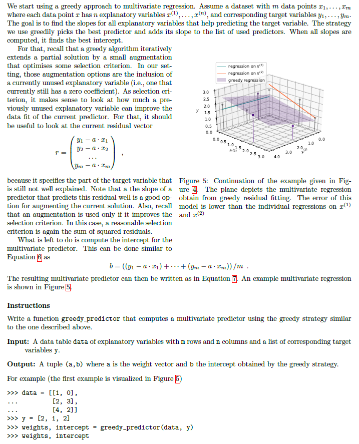
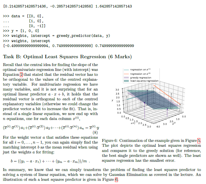
We start using a greedy approach to multivariate regression. Assume a dataset with m data points T1, ..., I'm where each data point r has n explanatory variables r(), ..., ("), and corresponding target variables y1, ..., ym. The goal is to find the slopes for all explanatory variables that help predicting the target variable. The strategy we use greedily picks the best predictor and adds its slope to the list of used predictors. When all slopes are computed, it finds the best intercept. For that, recall that a greedy algorithm iteratively extends a partial solution by a small augmentation that optimises some selection criterion. In our set- regression on x() ting, those augmentation options are the inclusion of regression on x(2) a currently unused explanatory variable (i.e., one that greedy regression currently still has a zero coefficient). As selection cri- 3.0 terion, it makes sense to look at how much a pre- 2.5 viously unused explanatory variable can improve the 20 data fit of the current predictor. For that, it should 15 10 be useful to look at the current residual vector 0.5 y1 - Q . T1 /2 - 0 . 12 10 051015202530 40 3.0 20 1.0 - 4 . I'm because it specifies the part of the target variable that Figure 5: Continuation of the example given in Fig- is still not well explained. Note that a the slope of a ure , The plane depicts the multivariate regression predictor that predicts this residual well is a good op- obtain from greedy residual fitting. The error of this tion for augmenting the current solution. Also, recall model is lower than the individual regressions on r() that an augmentation is used only if it improves the and r(2) selection criterion. In this case, a reasonable selection criterion is again the sum of squared residuals. What is left to do is compute the intercept for the multivariate predictor. This can be done similar to Equation 6 as b = ((y1 - a . ri) + + (Um - a . I'm)) /m . The resulting multivariate predictor can then be written as in Equation [7 An example multivariate regression is shown in Figure 5 Instructions Write a function greedy_predictor that computes a multivariate predictor using the greedy strategy similar to the one described above. Input: A data table data of explanatory variables with m rows and n columns and a list of corresponding target variables y. Output: A tuple (a, b) where a is the weight vector and b the intercept obtained by the greedy strategy. For example (the first example is visualized in Figure 5) >>> data = [[1, 0] , . . . [2, 3] , . . . [4, 2]] >>> y = [2, 1, 2] >>> weights, intercept = greedy_predictor (data, y) >>> weights, intercept[0 . 21428571428571436, -0. 2857142857142858] 1. 642857142857143 >>> data = [[0, 0] , [1, 0] , [0, -1]] > > > y = [i, 0, 0] >> weights, intercept = greedy_predictor (data, y) > >> weights, intercept [-0. 49999999999999994, 0. 74999999999999991 0.7499999999999999 Task B: Optimal Least Squares Regression (6 Marks) Recall that the central idea for finding the slope of the optimal univariate regression line (with intercept) was regression on x (4 Equation 2 that stated that the residual vector has to regression on x (2) be orthogonal to the values of the centred explanat greedy regression least squares regression tory variable. For multivariate regression we have many variables, and it is not surprising that for an 310 optimal linear predictor a . r + b, it holds that the 25 residual vector is orthogonal to each of the centred 20 explanatory variables (otherwise we could change the 15 1.0 predictor vector a bit to increase the fit). That is, in- 0.5 stead of a single linear equation, we now end up with n equations, one for each data column r(), 0.0 0510152025 30 40 2.0 1.0 0.0 (7( ) .1() ) ait(7(). 1(2)) a2+..+(x(i).p(")) an =I().y 3.0 (8) For the weight vector a that satisfies these equations for all i = 0, . .., n - 1, you can again simply find the Figure 6: Continuation of the example given in Figure 5 matching intercept b as the mean residual when using The plot depicts the optimal least squares regression just the weights a for fitting: and compares it to the greedy solution (for reference, the best single predictors are shown as well). The least b = ((y1 - a . ri) + ..+ (Um - a . Im))/m . squares regression has the smallest error. In summary, we know that we can simply transform the problem of finding the least squares predictor to solving a system of linear equation, which we can solve by Gaussian Elimination as covered in the lecture. An illustration of such a least squares predictor is given in Figure [6Instructions 1. Write a function equation (i, data, y) that produces the coefficients and the right-hand-side of the linear equation for explanatory variable r() (as specified in Equation (8)). Input: Integer i with 0 0 and n > 0, and list of target values y of length n. Output: Pair (c, d) where c is a list of coefficients of length n and d is a float representing the coefficients and right-hand-side of Equation S for data column i. For example (see Figure 6): > > > data = [[1, 0] , . . . [2, 3] , . . . [4, 2]] > > target = [2, 1, 2] > >> equation(0, data, target) ([4 . 666666666666666, 2.3333333333333326], 0.3333333333333326) >>> equation(1, data, target) ( [2.333333333333333, 4.666666666666666], -1.3333333333333335) 2. Write a function least_squares_predictor (data, y) that finds the optimal least squares predictor for the given data matrix and target vector. Input: Data matrix data with m rows and n columns such that m > 0 and n > 0. Output: Optimal predictor (a, b) with weight vector a (len(a)==n) and intercept b such that a, b minimise the sum of squared residuals. For Example: > >> data = [[0, 0], . . . [1, 0] , [0, -1] ] > >> y = [1, 0, 0] > >> weights, intercept = least_squares_predictor (data, y) >>> weights, intercept ([-0. 9999999999999997, 0. 9999999999999997], 0. 9999999999999998) > >> data = [[1, 0], . . . [2, 3] , . . . [4, 2]] >>> y = [2, 1, 2] > >> weights, intercept = least_squares_predictor(data, y) > >> weights, intercept (TO . 2857142857142855, -0. 42857142857142851 , 1. 7142857142857149)Country |Adult Mort infant dea percentage Hepatitis E Measles BMI under-five Polio Diphtheria HIV/AIDS GDP Population thinness 1 thinness 5- Schooling Life expectancy Liberia 29.95 74.52 25.97 76 0 24 11 75 76 1.1 3.26E+09 5057681 5.7 9.8 61.1 Monteneg 15.34 18.5 9 0 6.7 0 94 94 0.1 5.5E+09 628066 1.8 1.9 15.1 75.8 Rwanda 35.31 64.04 18.94 98 17 22.1 17 98 98 0.5 9.51E+09 12952218 5.9 4.9 10.8 65.2 Georgia 18.23 15.17 25.69 96 7872 27.1 1 94 93 0.1 1.76E+10 3989167 2.7 2.8 13.5 74.5 Armenia 18.69 1 25.71 95 10 53.3 1 96 95 0.1 1.24E+10 2989359 4.1 13.7 74.4 Mexico 30.73 17.29 20.99 82 0 28.1 37 83 83 0.1 1.22E+12 1.29E+08 1.6 1.9 13.9 76.6 Cyprus 10.32 0 36.61 96 0 59.2 0 99 99 0.1 2.5E+10 1207359 2.1 15.8 81 Samoa 21.99 0 22.99 0 73.8 0 62 67 0.1 8.21E+11 198414 1.2 1.1 13.9 73.6 Guyana 44.44 0 17.84 98 0 45 1 98 98 0.3 3.88E+09 786552 4.5 4.3 65.9 Bosnia and 14.35 0 35.33 91 0 54.7 0 87 89 0.1 2.02E+10 3280819 2.4 2.8 14.2 77 Uzbekistan 27.18 17 18.41 99 0 43 19 99 99 0.1 5.05E+10 33469203 3 3.1 11 69.1 Madagasci 33.8 29 10.62 74 6 19.5 40 73 74 0.4 1.39E+10 27691018 7.3 7.2 64.7 Paraguay 32.24 3 20.7 86 0 48.6 3 8 86 0.2 4.05E+10 7132538 2 2.9 13.3 73.8 Austria 10.77 4.32 45.57 95 0 25.4 0 95 95 0.1 4.55E+11 9006398 2 81.1 Morocco 17.48 18 23.22 99 92 56.5 21 99 99 0.1 1.18E+11 36910560 6.4 6.2 12.1 73.9 Guinea 27.38 27 16.27 63 53 22.2 41 63 63 1 1.09E+10 13132795 6.7 6.6 8.5 58.8 Guatemala 35.55 11 11.84 85 0 49.3 13 84 85 0.4 7.85E+10 17915568 2.2 2.3 13.7 71.4 Lesotho 53.42 4 40.34 93 516 31.4 6 9 93 9.6 2.74E+09 2142249 5.1 5.9 8.1 52.1 Argentina 18.78 8 26.31 94 0 61.6 10 99 94 0.1 5.20E+11 42539925 1 1.9 17.3 76 Botswana 46.47 2 25.81 95 36.8 2 96 95 2.8 1.86E+10 2351627 8 7.7 11.6 64.2