Question

1 Approved Answer

Posted on Oct 15, 2024

The places that require your code answer are marked with# YOUR CODEcomments. 1) Dimensionality Reduction The curse of dimensionality is an issue for many applications;

The places that require your code answer are marked with"# YOUR CODE"comments.

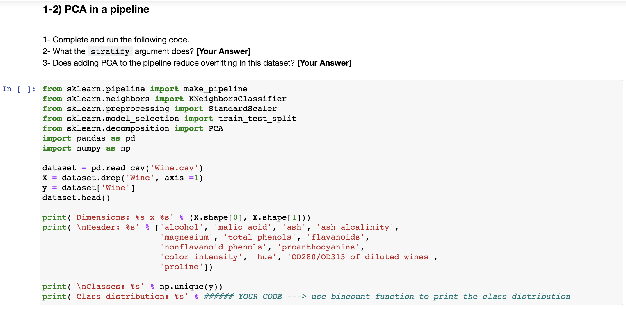
1) Dimensionality Reduction

The curse of dimensionality is an issue for many applications; increasing the number of features will not always improve classification accuracy. Dimensionality reduction techniques can help with the issue. The goal is to choose an optimum set of features of lower dimensionality to improve classification accuracy. These techniques fall into two major categories:

Feature selection:chooses a subset of the original features

Feature extraction:finds a set of new features (i.e., through some mapping f()) from the existing features

Principle Component Analysis (PCA)is a feature extraction technique that can be used to both compression (reduce the memory needed to store the data, speed up learning algorithm) and visualization.

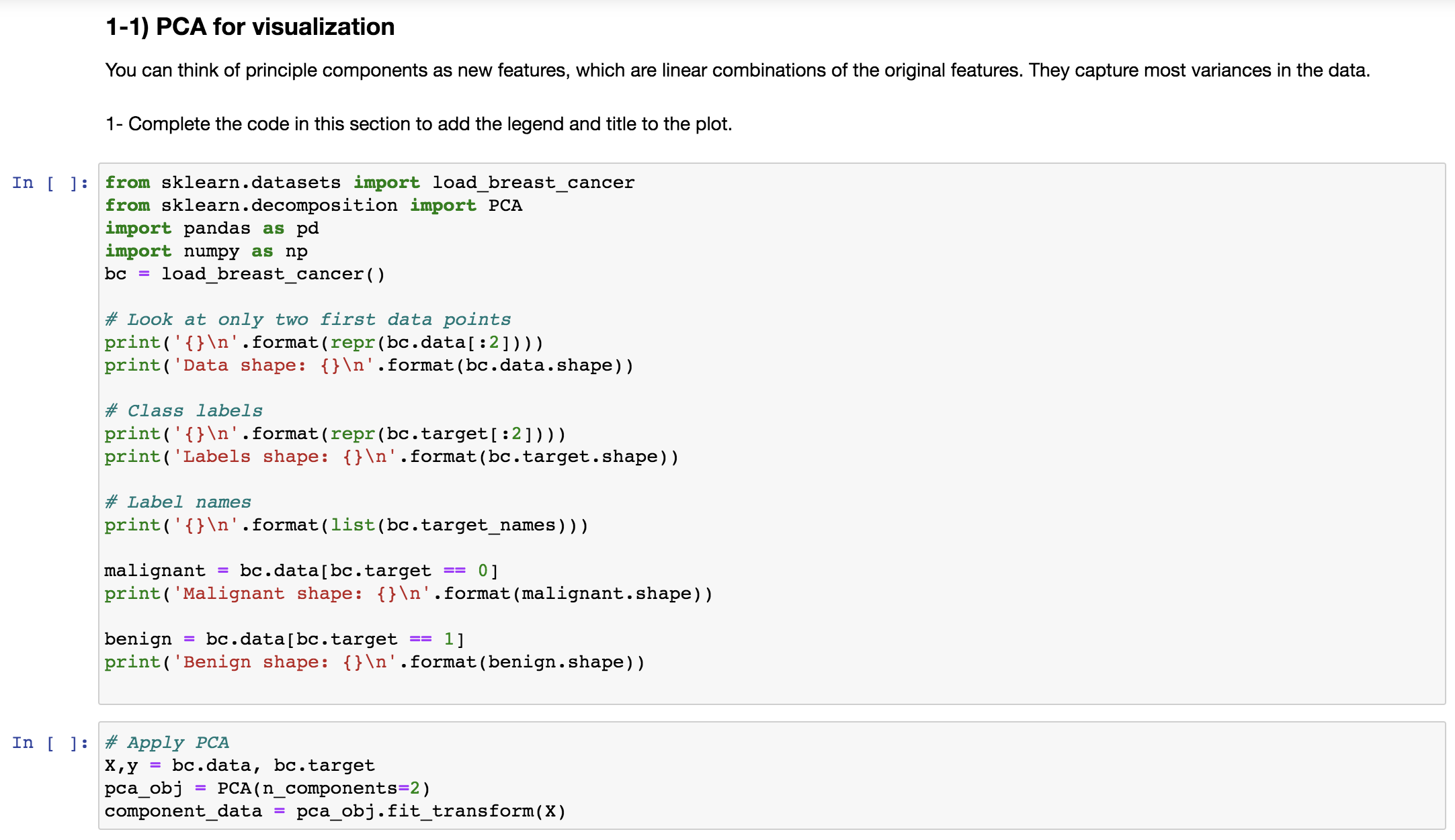
1-1) PCA for visualization

You can think of principle components as new features, which are linear combinations of the original features. They capture most variances in the data.

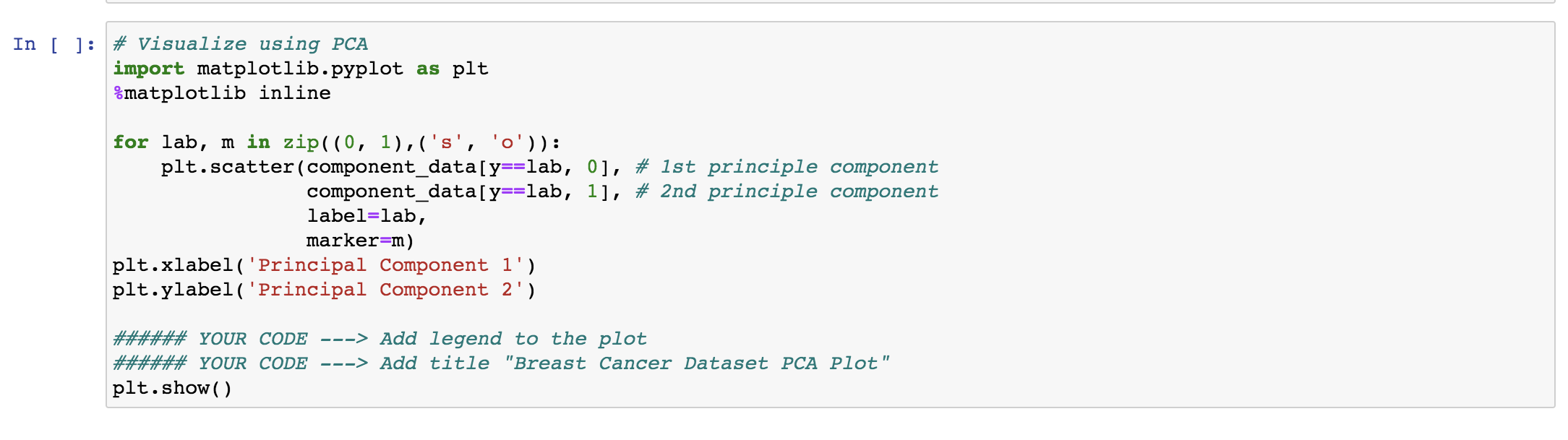
1- Complete the code in this section to add the legend and title to the plot.

1-1) PCA for visualization You can think of principle components as new features, which are linear combinations of the original features. They capture most variances in the data. 1- Complete the code in this section to add the legend and title to the plot. In [ ] : from sklearn . datasets import load_breast_cancer from sklearn . decomposition import PCA import pandas as pd import numpy as np bc = load_breast_cancer ( ) # Look at only two first data points print( ' {}\ ' . format (repr (bc . data[ : 2] ) ) ) print ( 'Data shape: {} \ ' . format (bc . data . shape) ) # Class labels print ( ' {}\ ' . format (repr (bc . target [ :2] ) ) ) print ( 'Labels shape: {}\ ' . format (bc . target . shape) ) # Label names print( ' {}\ ' . format (list (bc. target_names ) ) ) malignant = bc . data [bc . target == 0] print( 'Malignant shape: {}\ ' . format (malignant . shape) ) benign = bc . data [bc . target == 1] print ( 'Benign shape: {}\ ' . format (benign . shape) ) In [ ] : # Apply PCA X,y = bc. data, bc. target pca_obj = PCA(n_components=2) component_data = pca_obj . fit_transform(X)In [ ] : # Visualize using PCA import matplotlib. pyplot as plt :matplotlib inline for lab, m in zip( (0, 1) , ('s', 'o')) : plt . scatter (component_data [y==lab, 0], # 1st principle component component_data[y==lab, 1], # 2nd principle component label=lab, marker=m) pit. xlabel ( 'Principal Component 1' ) pit. ylabel ( 'Principal Component 2' ) ###### YOUR CODE ---> Add legend to the plot ##### YOUR CODE ---> Add title "Breast Cancer Dataset PCA Plot" pit . show ( )1-2) PCA in a pipeline 1- Complete and run the following code. 2- What the stratify argument does? [Your Answer] 3- Does adding PCA to the pipeline reduce overfitting in this dataset? [Your Answer] In [ ] : from sklearn . pipeline import make_pipeline from sklearn . neighbors import KNeighborsClassifier from sklearn . preprocessing import StandardScaler from sklearn.model_selection import train_test_split from sklearn . decomposition import PCA import pandas as pd import numpy as np dataset = pd. read_csv( 'Wine.csv' ) X = dataset . drop( 'Wine' , axis =1) y = dataset [ 'Wine' ] dataset . head ( ) print ( ' Dimensions: $s x $s' : (X. shape [0], X. shape[1]) ) print ( 'nHeader: $s' : ['alcohol', 'malic acid', 'ash', 'ash alcalinity', 'magnesium' , 'total phenols', 'flavanoids', 'nonflavanoid phenols' , 'proanthocyanins', 'color intensity', 'hue', 'OD280/0D315 of diluted wines', 'proline' ]) print ( ' \ Classes: $s' : np. unique(y) ) print ( 'Class distribution: $s' & ###### YOUR CODE ---> use bincount function to print the class distributionIn [ ]: X_train, X_test, y_train, y_test = train_test_split(X, y, random_state=123, test_size=0.3, stratify=y) pipe = make_pipeline (StandardScaler ( ) , KNeighborsClassifier (n_neighbors=5) ) pipe. fit (X_train, y_train) print( 'Orig. training accuracy: 8.2f$8' 8 (pipe. score(X_train, y_train) *100) ) print ( 'Orig. test accuracy: 8.2f:' 8 (pipe. score(X_test, y_test) *100) ) In [ ] : pipe_pca = make_pipeline (StandardScaler( ) , PCA (n_components=3) , KNeighborsClassifier (n_neighbors=5) ) pipe_pca . fit (X_train, y_train) print ( 'Transf. training accuracy: 8.2f$8' 8 (pipe_pca. score(X_train, y_train) *100) ) print ( 'Transf. test accuracy: 8.2f$8' 8 (pipe_pca. score(X_test, y_test) *100) )