Nesting function project with conditional formatting

Definition:

Nesting functions allows for multiple calculations to take place in a single cell.

Conditional Formatting selects one or more cells, and creates rules (conditions) for when and how those cells are formatted. The conditions can be, based on the selected cell's contents, or based on the contents of another cell.

This is a very tricky project but once mastered, you will be an expert on nesting functions. Please read the instructions carefully and use the referenced videos.

You will need to use an IF statement to determine the value of the letter grade.

An IF statement consists of a condition, a true value, and else value

For example:

In Cell D4 type: =IF(C2=6,"Hello","goodbye")

Place 6 in C2

Now change the value to 2

What does this mean.... If the value in cell C2 is equal 6 then the word "Hello" will display in cell D4. If the value is not 6 in C2 the "goodbye" will display in D4

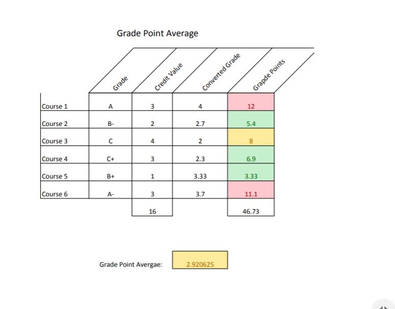
Project specification: Recreate the Project #1 PDF example

1. In cell C5 through C10 place the titles course 1 through 6).

2. In cell D4 through G4 place the titles Grade, Credit Value, Converted Grade, Grade Points

3. On the upper task bar select Format. Select cells. Align the cells D4 through G4 to a 45 degree angle.

4. Enter the values in D5 through E10 as stated in the recreation pdf.

5. Column F - converted Grade. This is where you will use a nested IF statement to determine the Grade point value. See table below: If this condition is met, then this, else, if this condition is met, then this, else, etc..... see example below

A = 4.00 grade points

A- = 3.70 grade points

B+ = 3.33 grade points

B = 3.00 grade points

B- = 2.70 grade points

C+ = 2.30 grade points

C = 2.00 grade points

D = 1.00 grade points

Below a D is 0 grade points

6. Column G: Grade Points is the product of Credit Value and Converted Grade.

7. Total the Credit Value and Grade Point Value

8. In F14 calculate the Grade Point Average: Formula - total grade points/ credit value

9. Conditional Formatting: Set up conditional formatting with the following criteria:

This is for cells G5 through G10

11 through 20 - Green color fill

7 through 10.9 - Yellow color fill

0 through 6.9 - Red color fill

See below for specific details on conditional formatting

10. Cell F14 should have conditional formatting with the following criteria:

3 to 4 - Green

2 to 2.9 - Yellow

0 to 1.9 - Red

11. When you are finished, please save the file as lastname_Project1.xlsx and submit file to the Week 3 Project 1 folder.

12. If you have and questions or you would like me to look at your project before submittal, please send the file to my email at no later than Friday, January 30, 2015 at noon.

IF statement nesting (column F)

To find Functions: Select the Formulas tab.

1. The first icon will provide you with a quick reference to all.

2. The AutoSum icon is a quick function to add up a column

3. Formula Builder icon takes you through step-by-step creation of the function

4. Reference icon will explain each of functions capabilities.

Use the formula builder to begin the nesting of the IF function for Column F (Converted Grade)

=IF(B5="A",4,IF(B5="A-",3.7,"continue with nesting for each of the conditions"))

Conditional Formatting for Column G - Start in G5 cell

To find Conditional Formatting: Select the Home tab

If you select the drop down arrow, a drop down box with option appears.

Select New Rule, There are several STYLEs to select from. Choose Classic

View the drop down boxes and select the following:

Select "Format only Cells that contain"

Select "Cell value"

Select "between" enter the values

Select format with " color value"

Select "OK"

Select the "+" to enter the New Rule, repeat until all conditions are entered.

Repeat through G10

Please seek additional help from your book or the Internet.

Grade Point Average Course 1 Course2 Course 3 Course 4 Course5 Course6 4 12 2.7 4 2.3 3.33 3.7 6.9 3.33 A- 11.1 16 46.73 Grade Point Avergae: 2.920625 Grade Point Average Course 1 Course2 Course 3 Course 4 Course5 Course6 4 12 2.7 4 2.3 3.33 3.7 6.9 3.33 A- 11.1 16 46.73 Grade Point Avergae: 2.920625