Neural network
Please formulate this data on SAS or Python with comments
The article is by James M. Hutchinson "A Nonparametric Approach to Pricing and Hedging Derivative Securities Via Learning Networks".
Just do as the pictures say, don't fit the neural network yet. just simulate data.


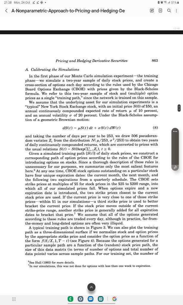
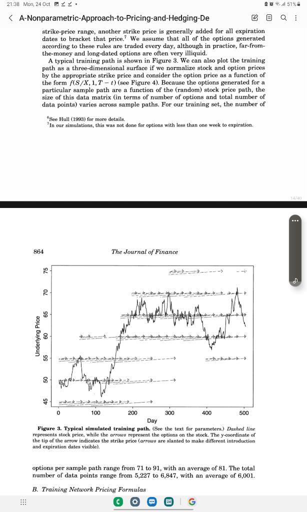
21:38 Mon, 240 oct b S(0) of $50, an and an annual volatility of 20 percent. Under the Black-Scholes assumption of a geometric Brownian motion: dS(t)=S(t)dt+S(t)dW(t) and taking the number of days per year to be 253, we draw 506 pseudorandom variates Zt from the distribution N(/253,2/253) to obtain two years of daily continuously compounded returns, which are converted to prices with the usual relations S(t)=S(0)exp(i1tZi),t0. Given a simulated training path {S(t)} of daily stock prices, we construct a corresponding path of option prices according to the rules of the CBOE for introducing options on stocks. Since a thorough description of these rules is unnecessary for our purposes, we summarize only the most salient features here. 6 At any one time, CBOE stock options outstanding on a particular stock have four unique expiration dates: the current month, the next month, and the following two expirations from a quarterly schedule. The CBOE sets strike prices at multiples of \$5 for stock prices in the $25 to $200 range, into which all of our simulated prices fall. When options expire and a new expiration date is introduced, the two strike prices closest to the current stock price are used. If the current price is very close to one of those strike prices-within $1 in our simulations-a third strike price is used to better bracket the current price. If the stock price moves outside of the current strike-price range, another strike price is generally added for all expiration dates to bracket that price. 7 We assume that all of the options generated according to these rules are traded every day, although in A typical training path is shown in Figure 3 . We can also plot the training path as a three-dimensional surface if we normalize stock and option prices by the appropriate strike price and consider the option price as a function of the form f(S/X,1,Tt) (see Figure 4). Because the options generated for a particular sample path are a function of the (random) stock price path, the size of this data matrix (in terms of number of options and total number of data points) varies across sample paths. For our training set, the number of 6 See Hull (1993) for more details. 7 In our simulations, this was not done for options with less than one week to expiration. strike-price range, another strike price is generally added for all expiration dates to bracket that price. 7 We assume that all of the options generated according to these rules are traded every day, although in practice, far-fromthe-money and long-dated options are often very illiquid. A typical training path is shown in Figure 3 . We can also plot the training path as a three-dimensional surface if we normalize stock and option prices by the appropriate strike price and consider the option price as a function of the form f(S/X,1,Tt ) (see Figure 4). Because the options generated for a particular sample path are a function of the (random) stock price path, the size of this data matrix (in terms of number of options and total number of data points) varies across sample paths. For our training set, the number of 6 See Hull (1993) for more details. In our simulations, this was not done for options with less than one week to expiration. 864 The Journal of Finance Figure 3. Typical simulated training path. (See the text for parameters.) Dashed line represents stock price, while the arrows represent the options on the stock. The y-coordinate of the tip of the arrow indicates the strike price (arrows are slanted to make different introduction and expiration dates visible). options per sample path range from 71 to 91 , with an average of 81 . The total number of data points range from 5,227 to 6,847 , with an average of 6,001 . 21:38 Mon, 240 oct b S(0) of $50, an and an annual volatility of 20 percent. Under the Black-Scholes assumption of a geometric Brownian motion: dS(t)=S(t)dt+S(t)dW(t) and taking the number of days per year to be 253, we draw 506 pseudorandom variates Zt from the distribution N(/253,2/253) to obtain two years of daily continuously compounded returns, which are converted to prices with the usual relations S(t)=S(0)exp(i1tZi),t0. Given a simulated training path {S(t)} of daily stock prices, we construct a corresponding path of option prices according to the rules of the CBOE for introducing options on stocks. Since a thorough description of these rules is unnecessary for our purposes, we summarize only the most salient features here. 6 At any one time, CBOE stock options outstanding on a particular stock have four unique expiration dates: the current month, the next month, and the following two expirations from a quarterly schedule. The CBOE sets strike prices at multiples of \$5 for stock prices in the $25 to $200 range, into which all of our simulated prices fall. When options expire and a new expiration date is introduced, the two strike prices closest to the current stock price are used. If the current price is very close to one of those strike prices-within $1 in our simulations-a third strike price is used to better bracket the current price. If the stock price moves outside of the current strike-price range, another strike price is generally added for all expiration dates to bracket that price. 7 We assume that all of the options generated according to these rules are traded every day, although in A typical training path is shown in Figure 3 . We can also plot the training path as a three-dimensional surface if we normalize stock and option prices by the appropriate strike price and consider the option price as a function of the form f(S/X,1,Tt) (see Figure 4). Because the options generated for a particular sample path are a function of the (random) stock price path, the size of this data matrix (in terms of number of options and total number of data points) varies across sample paths. For our training set, the number of 6 See Hull (1993) for more details. 7 In our simulations, this was not done for options with less than one week to expiration. strike-price range, another strike price is generally added for all expiration dates to bracket that price. 7 We assume that all of the options generated according to these rules are traded every day, although in practice, far-fromthe-money and long-dated options are often very illiquid. A typical training path is shown in Figure 3 . We can also plot the training path as a three-dimensional surface if we normalize stock and option prices by the appropriate strike price and consider the option price as a function of the form f(S/X,1,Tt ) (see Figure 4). Because the options generated for a particular sample path are a function of the (random) stock price path, the size of this data matrix (in terms of number of options and total number of data points) varies across sample paths. For our training set, the number of 6 See Hull (1993) for more details. In our simulations, this was not done for options with less than one week to expiration. 864 The Journal of Finance Figure 3. Typical simulated training path. (See the text for parameters.) Dashed line represents stock price, while the arrows represent the options on the stock. The y-coordinate of the tip of the arrow indicates the strike price (arrows are slanted to make different introduction and expiration dates visible). options per sample path range from 71 to 91 , with an average of 81 . The total number of data points range from 5,227 to 6,847 , with an average of 6,001
