Question: New Perspectives Excel 2016 | Module 4: SAM Mac Project la sam Inception Workspace ANALYZING AND CHARTING FINANCIAL DATA GETTING STARTED Open the file NP_EX16_Mac_4a_FirstLastName_1.xlsx,
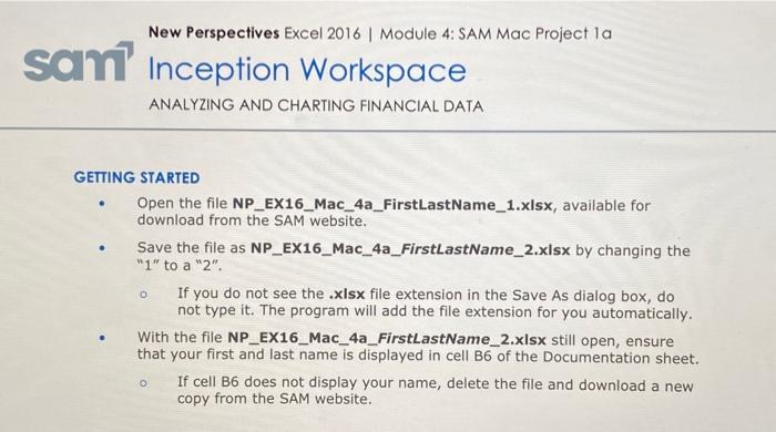
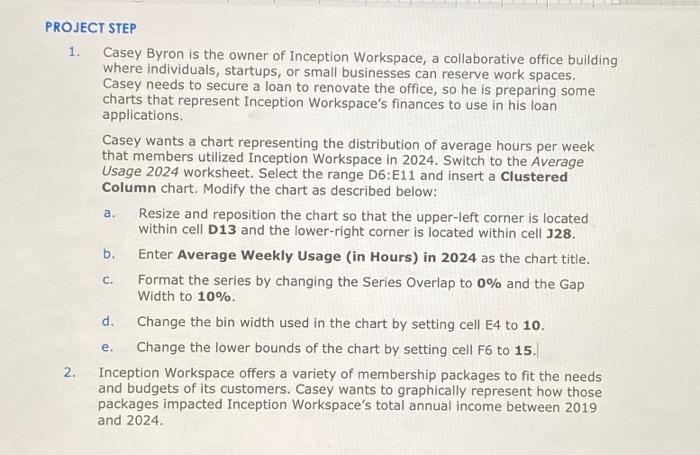
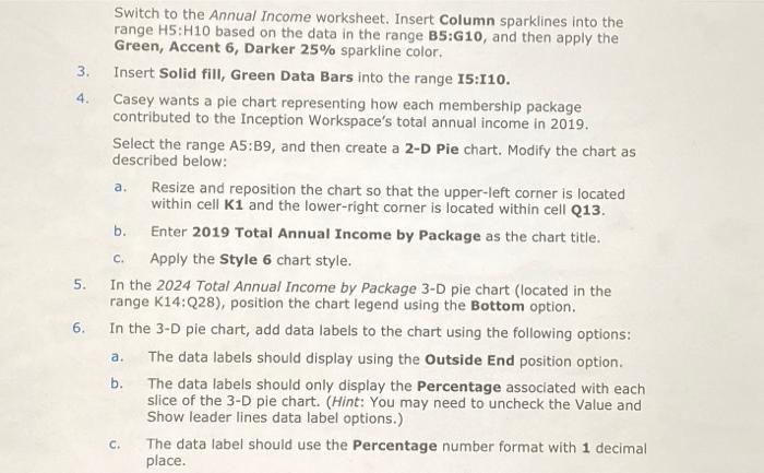
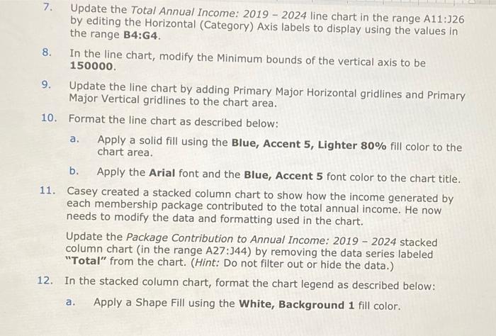
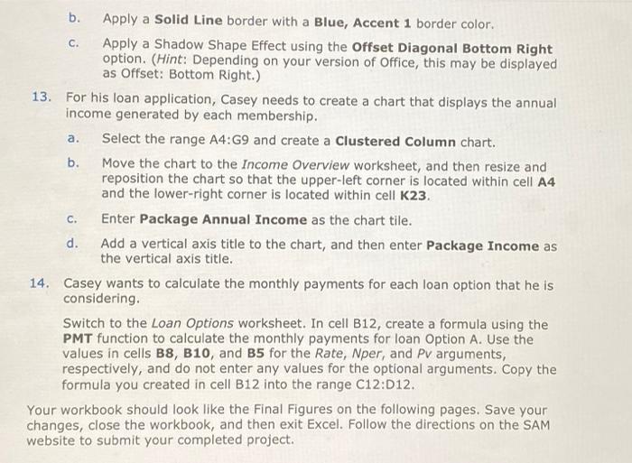
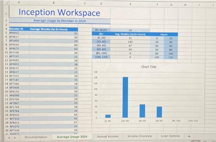
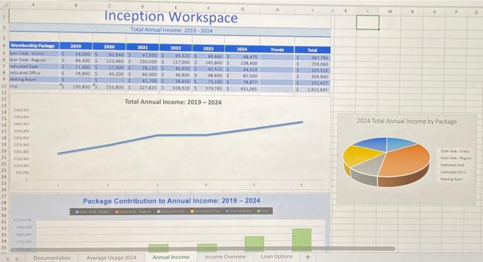
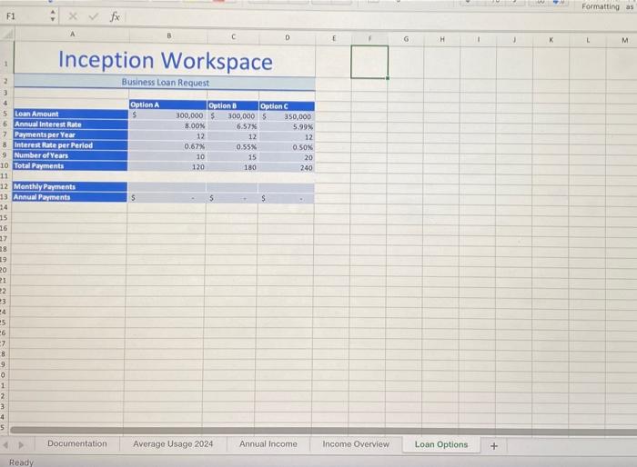
New Perspectives Excel 2016 | Module 4: SAM Mac Project la sam Inception Workspace ANALYZING AND CHARTING FINANCIAL DATA GETTING STARTED Open the file NP_EX16_Mac_4a_FirstLastName_1.xlsx, available for download from the SAM website. Save the file as NP_EX16_Mac_4a_FirstLastName_2.xlsx by changing the "1" to a "2" If you do not see the .xlsx file extension in the Save As dialog box, do not type it. The program will add the file extension for you automatically. With the file NP_EX16_Mac_4a_FirstLastName_2.xlsx still open, ensure that your first and last name is displayed in cell B6 of the Documentation sheet. If cell B6 does not display your name, delete the file and download a new copy from the SAM website. o a. PROJECT STEP 1. Casey Byron is the owner of Inception Workspace, a collaborative office building where individuals, startups, or small businesses can reserve work spaces. Casey needs to secure a loan to renovate the office, so he is preparing some charts that represent Inception Workspace's finances to use in his loan applications. Casey wants a chart representing the distribution of average hours per week that members utilized Inception Workspace in 2024. Switch to the Average Usage 2024 worksheet. Select the range D6:E11 and insert a Clustered Column chart. Modify the chart as described below: Resize and reposition the chart so that the upper-left corner is located within cell D13 and the lower-right corner is located within cell J28. b. Enter Average Weekly Usage (in Hours) in 2024 as the chart title. Format the series by changing the Series Overlap to 0% and the Gap Width to 10% d. Change the bin width used in the chart by setting cell E4 to 10. Change the lower bounds of the chart by setting cell F6 to 15. 2. Inception Workspace offers a variety of membership packages to fit the needs and budgets of its customers. Casey wants to graphically represent how those packages impacted Inception Workspace's total annual income between 2019 and 2024. C. e. 3. 4. a. Switch to the Annual Income worksheet. Insert Column sparklines into the range H5:H10 based on the data in the range B5:410, and then apply the Green, Accent 6, Darker 25% sparkline color. Insert Solid fill, Green Data Bars into the range 15:110. Casey wants a pie chart representing how each membership package contributed to the Inception Workspace's total annual income in 2019. Select the range AS:B9, and then create a 2-D Pie chart. Modify the chart as described below: Resize and reposition the chart so that the upper-left corner is located within cell K1 and the lower-right corner is located within cell Q13. b. Enter 2019 Total Annual Income by Package as the chart title. Apply the Style 6 chart style. In the 2024 Total Annual Income by Package 3-D pie chart (located in the range K14:Q28), position the chart legend using the Bottom option. In the 3-D pie chart, add data labels to the chart using the following options: a. The data labels should display using the Outside End position option. b. The data labels should only display the Percentage associated with each slice of the 3-D pie chart. (Hint: You may need to uncheck the value and Show leader lines data label options.) The data label should use the Percentage number format with 1 decimal place. c. 5. 6. C. a. 7. Update the Total Annual Income: 2019 - 2024 line chart in the range A11:26 by editing the Horizontal (Category) Axis labels to display using the values in the range B4:G4. 8. In the line chart, modify the Minimum bounds of the vertical axis to be 150000. 9. Update the line chart by adding Primary Major Horizontal gridlines and Primary Major Vertical gridlines to the chart area. 10. Format the line chart as described below: Apply a solid fill using the Blue, Accent 5, Lighter 80% fill color to the chart area. b. Apply the Arial font and the Blue, Accent 5 font color to the chart title. 11. Casey created a stacked column chart to show how the income generated by each membership package contributed to the total annual income. He now needs to modify the data and formatting used in the chart. Update the Package Contribution to Annual Income: 2019 - 2024 stacked column chart (in the range A27:344) by removing the data series labeled "Total" from the chart. (Hint: Do not filter out or hide the data.) 12. In the stacked column chart, format the chart legend as described below: Apply a Shape Fill using the White, Background 1 fill color. a. C. a. C. b. Apply a Solid Line border with a Blue, Accent 1 border color. Apply a Shadow Shape Effect using the Offset Diagonal Bottom Right option. (Hint: Depending on your version of Office, this may be displayed as Offset: Bottom Right.) 13. For his loan application, Casey needs to create a chart that displays the annual income generated by each membership. Select the range A4:49 and create a Clustered Column chart. b. Move the chart to the Income Overview worksheet, and then resize and reposition the chart so that the upper-left corner is located within cell A4 and the lower-right corner is located within cell K23. Enter Package Annual Income as the chart tile. d. Add a vertical axis title to the chart, and then enter Package Income as the vertical axis title. 14. Casey wants to calculate the monthly payments for each loan option that he is considering. Switch to the Loan Options worksheet. In cell B12, create a formula using the PMT function to calculate the monthly payments for loan Option A. Use the values in cells B8, B10, and B5 for the Rate, Nper, and Pv arguments, respectively, and do not enter any values for the optional arguments. Copy the formula you created in cell B12 into the range C12:012. Your workbook should look like the Final Figures on the following pages. Save your changes, close the workbook, and then exit Excel. Follow the directions on the SAM website to submit your completed project. A D E F G H Inception Workspace 2 Average Usage by Member in 2024 Bin Width Bin 10,20 120,40] [40.601 160,80) (80, 1001 1100, 1201 20 Avg. Weekly Use in Hours) 11 142 47 39 0 0 0 20 40 60 80 100 Hours 20 40 60 80 100 120 Chart Title 160 160 3 4 Member ID SAP6052 6 AP9617 7 AP5409 8 AP9034 9 AP9673 10 AP3708 11 AP2235 12 AP9499 13 AP5853 14 AP8225 15 AP8617 16 AP7315 17 AP7187 18 AP7346 19 AP5408 20 AP8150 21 AP6068 22 AP3706 23 AP7867 24 AP1744 25 AP9764 26 AP8020 27 AP7310 28 AP8013 29 AP1073 30 AP7539 21 AD002 Average Weekly Use in Hours) 32 30 29 60 63 30 22 29 28 25 21 33 35 28 22 33 22 29 20 58 26 66 43 67 26 26 31 Documentation Average Usage 2024 120 100 NO 60 40 20 0 1920) 120,40 140.60 160,80 01001 1100 1201 Annual Income Income Overview Loan Options + M O P Inception Workspace --- Total Annual income: 2019-2024 Trends To 2018 SE000 36.400 71 600 18.8005 5 11000 2020 52.60 120,960 27.000 43.2003 2021 2022 67,50035 505015 110,500 117,000 225 40,95023 50,000 45,800 41.700 5 $8.50 327,825 32.920 2023 2014 68.66035 68.475 145.800 158.400 2. 4313 48.6005 $2,500 73.2005 21.027 379,75 5 411,565 5. 362,795 5 750.00 201.31 $ 109.900 5 252427 $11.95 253.8005 Total Annual Income: 2019-2024 + Membership Package 3. Deko 3 6 en Dekor $ 7edicated De 5 edicated $ Metinom 5 10 15 11 12 13 14 15 16 17 100 15 19 120.000 20 21 22 23 24 25 26 27 2024 Total Annual income by Package OD De DO Package Contribution to Annual Income: 2019-2024 29 30 31 32 33 34 35 Documentation Average Usage 2024 Annual income Income Overview Loan Options + B D G H M N N o P 1 Inception Workspace Annual Income Overview: 2019-2024 2 3 4 5 6 7 8 9 10 11 12 13 14 15 16 17 18 19 20 21 22 23 24 25 26 27 28 29 30 31 32 33 35 Documentation Averago Usage 2024 Annual income Income Overview Loan Options + Ready Formatting as F1 fx B D H 1 1 K M 1 Inception Workspace - Business Loan Request Option A $ Option Option 300,000 $300,000 5 350,000 8.00% 6.57% 5.99% 12 12 12 0.67% 0.55% O.SOX 10 15 20 120 180 240 5 5 $ 2 3 4 5 Loan Amount 6 Annual interest Rate 7 Payments per Year 8 Interest Rate per Period 9 Number of Years 10 Total Payments 11 12 Monthly Payments 13 Annual Payments 24 15 16 17 38 19 20 21 22 3 24 5 6 7 8 9 0 1 2 3 4 5 Documentation Average Usage 2024 Annual Income Income Overview Loan Options + Ready New Perspectives Excel 2016 | Module 4: SAM Mac Project la sam Inception Workspace ANALYZING AND CHARTING FINANCIAL DATA GETTING STARTED Open the file NP_EX16_Mac_4a_FirstLastName_1.xlsx, available for download from the SAM website. Save the file as NP_EX16_Mac_4a_FirstLastName_2.xlsx by changing the "1" to a "2" If you do not see the .xlsx file extension in the Save As dialog box, do not type it. The program will add the file extension for you automatically. With the file NP_EX16_Mac_4a_FirstLastName_2.xlsx still open, ensure that your first and last name is displayed in cell B6 of the Documentation sheet. If cell B6 does not display your name, delete the file and download a new copy from the SAM website. o a. PROJECT STEP 1. Casey Byron is the owner of Inception Workspace, a collaborative office building where individuals, startups, or small businesses can reserve work spaces. Casey needs to secure a loan to renovate the office, so he is preparing some charts that represent Inception Workspace's finances to use in his loan applications. Casey wants a chart representing the distribution of average hours per week that members utilized Inception Workspace in 2024. Switch to the Average Usage 2024 worksheet. Select the range D6:E11 and insert a Clustered Column chart. Modify the chart as described below: Resize and reposition the chart so that the upper-left corner is located within cell D13 and the lower-right corner is located within cell J28. b. Enter Average Weekly Usage (in Hours) in 2024 as the chart title. Format the series by changing the Series Overlap to 0% and the Gap Width to 10% d. Change the bin width used in the chart by setting cell E4 to 10. Change the lower bounds of the chart by setting cell F6 to 15. 2. Inception Workspace offers a variety of membership packages to fit the needs and budgets of its customers. Casey wants to graphically represent how those packages impacted Inception Workspace's total annual income between 2019 and 2024. C. e. 3. 4. a. Switch to the Annual Income worksheet. Insert Column sparklines into the range H5:H10 based on the data in the range B5:410, and then apply the Green, Accent 6, Darker 25% sparkline color. Insert Solid fill, Green Data Bars into the range 15:110. Casey wants a pie chart representing how each membership package contributed to the Inception Workspace's total annual income in 2019. Select the range AS:B9, and then create a 2-D Pie chart. Modify the chart as described below: Resize and reposition the chart so that the upper-left corner is located within cell K1 and the lower-right corner is located within cell Q13. b. Enter 2019 Total Annual Income by Package as the chart title. Apply the Style 6 chart style. In the 2024 Total Annual Income by Package 3-D pie chart (located in the range K14:Q28), position the chart legend using the Bottom option. In the 3-D pie chart, add data labels to the chart using the following options: a. The data labels should display using the Outside End position option. b. The data labels should only display the Percentage associated with each slice of the 3-D pie chart. (Hint: You may need to uncheck the value and Show leader lines data label options.) The data label should use the Percentage number format with 1 decimal place. c. 5. 6. C. a. 7. Update the Total Annual Income: 2019 - 2024 line chart in the range A11:26 by editing the Horizontal (Category) Axis labels to display using the values in the range B4:G4. 8. In the line chart, modify the Minimum bounds of the vertical axis to be 150000. 9. Update the line chart by adding Primary Major Horizontal gridlines and Primary Major Vertical gridlines to the chart area. 10. Format the line chart as described below: Apply a solid fill using the Blue, Accent 5, Lighter 80% fill color to the chart area. b. Apply the Arial font and the Blue, Accent 5 font color to the chart title. 11. Casey created a stacked column chart to show how the income generated by each membership package contributed to the total annual income. He now needs to modify the data and formatting used in the chart. Update the Package Contribution to Annual Income: 2019 - 2024 stacked column chart (in the range A27:344) by removing the data series labeled "Total" from the chart. (Hint: Do not filter out or hide the data.) 12. In the stacked column chart, format the chart legend as described below: Apply a Shape Fill using the White, Background 1 fill color. a. C. a. C. b. Apply a Solid Line border with a Blue, Accent 1 border color. Apply a Shadow Shape Effect using the Offset Diagonal Bottom Right option. (Hint: Depending on your version of Office, this may be displayed as Offset: Bottom Right.) 13. For his loan application, Casey needs to create a chart that displays the annual income generated by each membership. Select the range A4:49 and create a Clustered Column chart. b. Move the chart to the Income Overview worksheet, and then resize and reposition the chart so that the upper-left corner is located within cell A4 and the lower-right corner is located within cell K23. Enter Package Annual Income as the chart tile. d. Add a vertical axis title to the chart, and then enter Package Income as the vertical axis title. 14. Casey wants to calculate the monthly payments for each loan option that he is considering. Switch to the Loan Options worksheet. In cell B12, create a formula using the PMT function to calculate the monthly payments for loan Option A. Use the values in cells B8, B10, and B5 for the Rate, Nper, and Pv arguments, respectively, and do not enter any values for the optional arguments. Copy the formula you created in cell B12 into the range C12:012. Your workbook should look like the Final Figures on the following pages. Save your changes, close the workbook, and then exit Excel. Follow the directions on the SAM website to submit your completed project. A D E F G H Inception Workspace 2 Average Usage by Member in 2024 Bin Width Bin 10,20 120,40] [40.601 160,80) (80, 1001 1100, 1201 20 Avg. Weekly Use in Hours) 11 142 47 39 0 0 0 20 40 60 80 100 Hours 20 40 60 80 100 120 Chart Title 160 160 3 4 Member ID SAP6052 6 AP9617 7 AP5409 8 AP9034 9 AP9673 10 AP3708 11 AP2235 12 AP9499 13 AP5853 14 AP8225 15 AP8617 16 AP7315 17 AP7187 18 AP7346 19 AP5408 20 AP8150 21 AP6068 22 AP3706 23 AP7867 24 AP1744 25 AP9764 26 AP8020 27 AP7310 28 AP8013 29 AP1073 30 AP7539 21 AD002 Average Weekly Use in Hours) 32 30 29 60 63 30 22 29 28 25 21 33 35 28 22 33 22 29 20 58 26 66 43 67 26 26 31 Documentation Average Usage 2024 120 100 NO 60 40 20 0 1920) 120,40 140.60 160,80 01001 1100 1201 Annual Income Income Overview Loan Options + M O P Inception Workspace --- Total Annual income: 2019-2024 Trends To 2018 SE000 36.400 71 600 18.8005 5 11000 2020 52.60 120,960 27.000 43.2003 2021 2022 67,50035 505015 110,500 117,000 225 40,95023 50,000 45,800 41.700 5 $8.50 327,825 32.920 2023 2014 68.66035 68.475 145.800 158.400 2. 4313 48.6005 $2,500 73.2005 21.027 379,75 5 411,565 5. 362,795 5 750.00 201.31 $ 109.900 5 252427 $11.95 253.8005 Total Annual Income: 2019-2024 + Membership Package 3. Deko 3 6 en Dekor $ 7edicated De 5 edicated $ Metinom 5 10 15 11 12 13 14 15 16 17 100 15 19 120.000 20 21 22 23 24 25 26 27 2024 Total Annual income by Package OD De DO Package Contribution to Annual Income: 2019-2024 29 30 31 32 33 34 35 Documentation Average Usage 2024 Annual income Income Overview Loan Options + B D G H M N N o P 1 Inception Workspace Annual Income Overview: 2019-2024 2 3 4 5 6 7 8 9 10 11 12 13 14 15 16 17 18 19 20 21 22 23 24 25 26 27 28 29 30 31 32 33 35 Documentation Averago Usage 2024 Annual income Income Overview Loan Options + Ready Formatting as F1 fx B D H 1 1 K M 1 Inception Workspace - Business Loan Request Option A $ Option Option 300,000 $300,000 5 350,000 8.00% 6.57% 5.99% 12 12 12 0.67% 0.55% O.SOX 10 15 20 120 180 240 5 5 $ 2 3 4 5 Loan Amount 6 Annual interest Rate 7 Payments per Year 8 Interest Rate per Period 9 Number of Years 10 Total Payments 11 12 Monthly Payments 13 Annual Payments 24 15 16 17 38 19 20 21 22 3 24 5 6 7 8 9 0 1 2 3 4 5 Documentation Average Usage 2024 Annual Income Income Overview Loan Options + Ready
Step by Step Solution
There are 3 Steps involved in it

Get step-by-step solutions from verified subject matter experts


