NPV Worksheet: 50 points

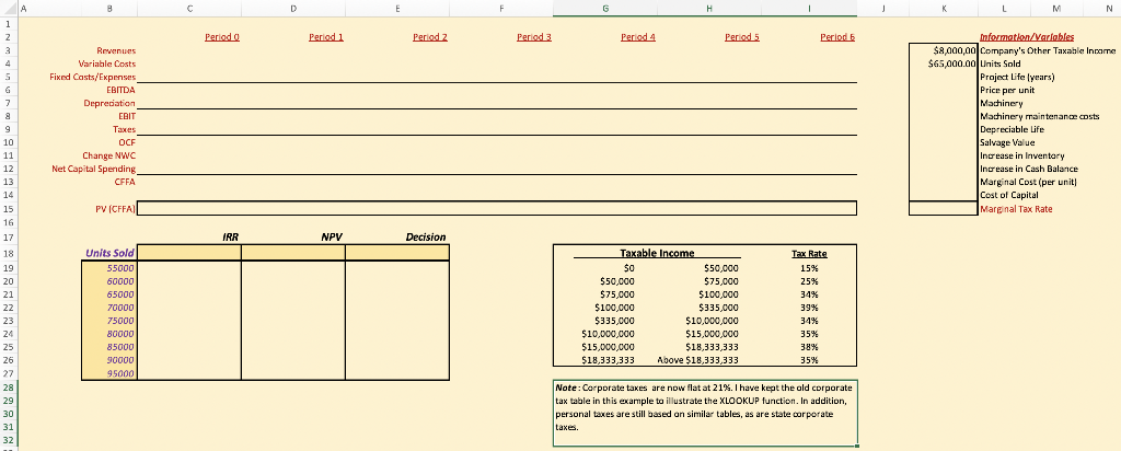
Garca and Martinez manufacture widgets and currently have $8 million in taxable income. The company is considering an expansion, and theyve asked you to evaluate the project. The expansion requires the firm to produce 65,000 widgets a year for 6 years, and the company estimates they can sell them for $30 per widget. Garca and Martinez estimate they will need an additional $4,000,000 worth of machinery. The machinery costs $120,000 a year to operate and maintain. The machinerys depreciable life is 7-years, and the company expects to salvage the machinery for $160,000 at the end of year 6. If the project is accepted, the company will immediately increase inventory by $500,000 and maintain the new inventory level over the projects life. Similarly, the company will immediately add $50,000 to their cash balance at start-up and then again in year 1 and maintain that higher cash balance over the projects life. The investments in cash and inventory will be recovered when the project is completed. The marginal cost of producing a widget is $6.00 and the cost of capital is 14%. Calculate the projects NPV by linking to the information/variable values in Column K.

1. Enter the relevant values for the variables that you use in solving this problem in Column K (as Ive done with the companys taxable income in K3 and the units sold in K4). Name each cell in Column K that contains a variable. (e.g. define the name of cell K4to be Quantity). Where possible (linking cells or writing functions), use these names to reference the cells in your calculations. This makes it easier for others to know what the functions are doing. (5 points)

2. Reformat Row 2 (cells C2 to I2) so that the numbers display the text Year instead of Period. For example, there is currently a zero in cell C2, but we see Period 0 displayed and not just 0. Change this so it displays as Year 0 (this formatting trick allows us to use the numbers in calculations, but we can also use labels so we know what the numbers represent). (3 points)

3. Calculate the net capital spending for each period in Row 12 and calculate the change in net working capital for each period in Row11. (5 points)

4. Calculate the operating cash flow for each period in Row 10.

a. Using relative and/or absolute cell references, use the VDB function in Row 7 to calculate depreciation. Note the function should use the accelerated (double-declining) depreciation for each year but switch to straight-line when its depreciation is larger. If done and linked correctly, whenI copy the cell in Column D into Column I, the cell in Column I will return the correct answer for depreciation. (3 points)

b. Use the XLOOKUP function on the provided tax table to calculate the marginal tax rate in cell K15. Use that marginal tax rate to calculate taxes in each year in Row 9. (3 points)

c. Make sure to fill in rows 3 to 9, and then calculate the OCF for each period in Row 10. (2 points)

5. Evaluate the project.

a. Calculate the cash flow from assets in Row 13. (2 points)

b. Using relative and/or absolute cell references, use the PV function to calculate the present value of CFFA for each year in Row 15. If done correctly, I will be able to copy cell C15 and paste it into cells D15:I15 and those cells will display the correct present value. (3 points)

c. Use the NPV function in D18 to calculate the net present value of the project. If done correctly, it will give the same value as summing cells C15 to I15. (3 points)

d. Use the IRR function in C18 to calculate the internal rate of return on the project. (3 points)

e. In E19, use an IF statement to return the text Accept or Reject depending on the NPV calculation. (2 points)

6. Construct a sensitivity analysis for units sold (quantities are listed in Column B starting in Row 19). Define a data table using Excels What-If Analysis located in the data tab. (6 points)

a. The table should include the IRR, NPV, and Decision for each quantity; i.e. for each quantity Excel will calculate these three items in the table which will extend from C19to E27. b.Use conditional formatting(found in the Home tab) to highlight the NPV in red if the NPV is negative, and green if it is positive.Use a conditional format to highlight the IRR in red if the IRR is greater than the cost of capital, and in green if it is less than the cost of capital.

7. Define abase-case, best-case and worst-case scenario using the Scenario Manager in Excels What-If Analysis. Use the following value ranges for the best and worst cases: (6 points)

a. Per unit price is plus/minus $5.

b. Quantity sold is plus/minus 15,000 units.

c. Marginal cost of producing a widget is plus/minus $1.508.Using the Scenario Manager, create a scenario summary. (4 points)

8. Using the Scenario Manager, create a scenario summary. (4 points)

A D E F G H M N Periodo Period 1 Period z Period 3 Period 4 Periods Period 1 z 3 4 Revenues Variable Costs Fixed Casts/Expenses EBITDA Depreciation EBIT Taxes OCE Change NWC Net Capital Spending CFFA Information/Variables $8,000,00 Company's Other Taxable income $65,000.00 Units Sold Project Life Cyears) Price per unit Machinery Machinery maintenance costs Depreciable Life Salvage Value Increase in Inventory Increase in Cash Balance Marginal Cost (per unit) Cost of Capital Marginal Tax Rate PV (CFFA IRR NPV Decision 6 7 a 9 10 11 12 13 14 15 16 17 18 19 20 21 22 23 24 25 26 22 28 29 30 31 32 Units Sold 55000 60000 65000 70000 75000 80000 85000 90000 95000 Tax Rate 15% 25% 34% 39% Taxable income $o $50,000 $50,000 $75,000 $75,000 $100,000 $100,000 $335,000 $ $335,000 $10,000,000 $10,000,000 $15,000,000 $15,000,000 $18,333,333 $18,333,333 Above $18,333,333 34% 35% 38% 35% Note: Corporate taxes are now flat at 21%. I have kept the old corporate tax table in this example to illustrate the XLOOKUP function. In addition, personal taxes are still based on similar tables, as are state corporate taxes. A D E F G H M N Periodo Period 1 Period z Period 3 Period 4 Periods Period 1 z 3 4 Revenues Variable Costs Fixed Casts/Expenses EBITDA Depreciation EBIT Taxes OCE Change NWC Net Capital Spending CFFA Information/Variables $8,000,00 Company's Other Taxable income $65,000.00 Units Sold Project Life Cyears) Price per unit Machinery Machinery maintenance costs Depreciable Life Salvage Value Increase in Inventory Increase in Cash Balance Marginal Cost (per unit) Cost of Capital Marginal Tax Rate PV (CFFA IRR NPV Decision 6 7 a 9 10 11 12 13 14 15 16 17 18 19 20 21 22 23 24 25 26 22 28 29 30 31 32 Units Sold 55000 60000 65000 70000 75000 80000 85000 90000 95000 Tax Rate 15% 25% 34% 39% Taxable income $o $50,000 $50,000 $75,000 $75,000 $100,000 $100,000 $335,000 $ $335,000 $10,000,000 $10,000,000 $15,000,000 $15,000,000 $18,333,333 $18,333,333 Above $18,333,333 34% 35% 38% 35% Note: Corporate taxes are now flat at 21%. I have kept the old corporate tax table in this example to illustrate the XLOOKUP function. In addition, personal taxes are still based on similar tables, as are state corporate taxes