Numerical Methods for Ordinary Differential Equations: Initial Value Problems
NOTE:
Python is required, not MATLAB.
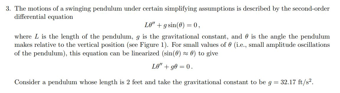
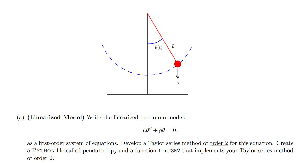
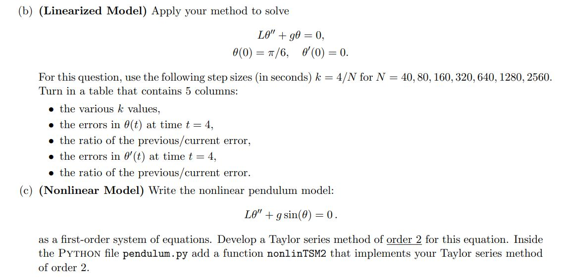
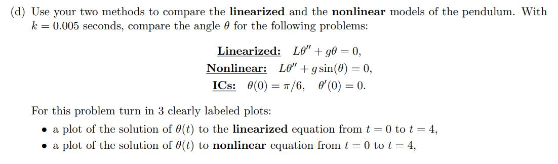
3. The motions of a swinging pendulum under certain simplifying assumptions is described by the second-order differential equation LO" +gsin(O) = 0, where L is the length of the pendulum, g is the gravitational constant, and is the angle the pendulum makes relative to the vertical position (see Figure 1). For small values of 0 (i.e., small amplitude oscillations of the pendulum), this equation can be linearized (sin(0) - 0) to give L" +90 = 0. Consider a pendulum whose length is 2 feet and take the gravitational constant to be g = 32.17 ft/s2. 0(t) L -- - (a) (Linearized Model) Write the linearized pendulum model: LO" + 0 = 0. as a first-order system of equations. Develop a Taylor series method of order 2 for this equation. Create a PYTHON file called pendulum.py and a function linTSM2 that implements your Taylor series method of order 2. (b) (Linearized Model) Apply your method to solve LO" +90 = 0, 0(0) = 1/6, 0'(0) = 0. For this question, use the following step sizes in seconds) k = 4/N for N = 40, 80, 160, 320, 640, 1280, 2560. Turn in a table that contains 5 columns: the various k values, the errors in 0(t) at time t = 4, the ratio of the previous/current error, the errors in 6'(t) at time t = 4, the ratio of the previous/current error. (c) (Nonlinear Model) Write the nonlinear pendulum model: LO" + g sin(0) = 0. as a first-order system of equations. Develop a Taylor series method of order 2 for this equation. Inside the PYTHON file pendulum.py add a function nonlin TSM2 that implements your Taylor series method of order 2. (d) Use your two methods to compare the linearized and the nonlinear models of the pendulum. With k= 0.005 seconds, compare the angle for the following problems: Linearized: LO" +90 = 0, Nonlinear: LO" + g sin(0) = 0, ICs: 0(0) = 7/6, 0'0) = 0. For this problem turn in 3 clearly labeled plots: a plot of the solution of (t) to the linearized equation from t=0 to t= 4, . a plot of the solution of 0(t) to nonlinear equation from t = 0 to t = 4, a plot that contains both solutions of (t) from t = 0 to t = 4. Make sure to include a legend for plot this plot. (e) What do these plots say about the validity of the linearized equation as an approximation to the nonlinear equation? 3. The motions of a swinging pendulum under certain simplifying assumptions is described by the second-order differential equation LO" +gsin(O) = 0, where L is the length of the pendulum, g is the gravitational constant, and is the angle the pendulum makes relative to the vertical position (see Figure 1). For small values of 0 (i.e., small amplitude oscillations of the pendulum), this equation can be linearized (sin(0) - 0) to give L" +90 = 0. Consider a pendulum whose length is 2 feet and take the gravitational constant to be g = 32.17 ft/s2. 0(t) L -- - (a) (Linearized Model) Write the linearized pendulum model: LO" + 0 = 0. as a first-order system of equations. Develop a Taylor series method of order 2 for this equation. Create a PYTHON file called pendulum.py and a function linTSM2 that implements your Taylor series method of order 2. (b) (Linearized Model) Apply your method to solve LO" +90 = 0, 0(0) = 1/6, 0'(0) = 0. For this question, use the following step sizes in seconds) k = 4/N for N = 40, 80, 160, 320, 640, 1280, 2560. Turn in a table that contains 5 columns: the various k values, the errors in 0(t) at time t = 4, the ratio of the previous/current error, the errors in 6'(t) at time t = 4, the ratio of the previous/current error. (c) (Nonlinear Model) Write the nonlinear pendulum model: LO" + g sin(0) = 0. as a first-order system of equations. Develop a Taylor series method of order 2 for this equation. Inside the PYTHON file pendulum.py add a function nonlin TSM2 that implements your Taylor series method of order 2. (d) Use your two methods to compare the linearized and the nonlinear models of the pendulum. With k= 0.005 seconds, compare the angle for the following problems: Linearized: LO" +90 = 0, Nonlinear: LO" + g sin(0) = 0, ICs: 0(0) = 7/6, 0'0) = 0. For this problem turn in 3 clearly labeled plots: a plot of the solution of (t) to the linearized equation from t=0 to t= 4, . a plot of the solution of 0(t) to nonlinear equation from t = 0 to t = 4, a plot that contains both solutions of (t) from t = 0 to t = 4. Make sure to include a legend for plot this plot. (e) What do these plots say about the validity of the linearized equation as an approximation to the nonlinear equation