Objective of the activity Use the script provided by the teacher to solve a diffusion problem in a ternary system with the Stefan-Maxwell equations.

Instructions a. Draw a diagram with the boundary conditions for example 1.17 from the book Principles and Modern Applications of Mass Transfer Operations by the author Jaime Benitez. b. Write the Stefan Maxwell equations for the ternary system stated in the example. c. Makes the variable changes specified in the example. d. Obtain an estimate of the initial values of the Na and Nb fluxes from the Fick's Law equations, using the effective diffusion coefficients for a multicomponent mixture. and. Use the script in MATLAB software to obtain the values of the fluxes Na and Nb and the concentration profiles of species a, b and c. F. Upload the results, graphs and screenshot of the use of the script to the Classroom platform.

example 1.17 from the book Principles and Modern Applications of Mass Transfer Operations by the author Jaime Benitez.

script provided to solve a diffusion problem in a ternary system with the Stefan-Maxwell equations.

function ydot=MaxwellStefan(t,y)

global N1 N2 N3

N3=0; F12 = 1.286e-3; F13 = 2.081e-3; F23 = 3.019e-3;

ydot(1)=(y(1)*N2-y(2)*N1)/F12+(y(1)*N3-(1-y(1)-y(2))*N1)/F13; ydot(2)=(y(2)*N1-y(1)*N2)/F12+(y(2)*N3-(1-y(1)-y(2))*N2)/F23;

ydot=ydot';

function f=shooting(N)

global N1 N2 N3

N1=N(1); N2=N(2);

[t,y]=ode45('MaxwellStefan',[0 1],[0.319 0.528]);

f(1)=y(end,1); f(2)=y(end,2);

global N1 N2 N3

N3=0;

N=fsolve('shooting',[0.001 0.001],optimset('TolFun',1e-10));

N1=N(1) N2=N(2)

[t,y]=ode45('MaxwellStefan',[0 1],[0.319 0.528]);

figure(1); hold on; Axis([0 1 0 1]); plot(t,y(:,1),'r') plot(t,y(:,2),'b') plot(t,1-y(:,1)-y(:,2),'g')

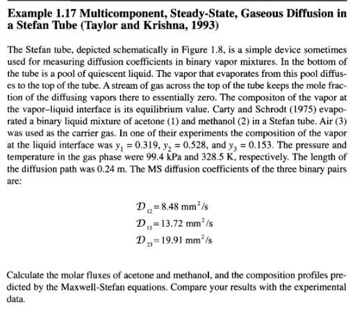
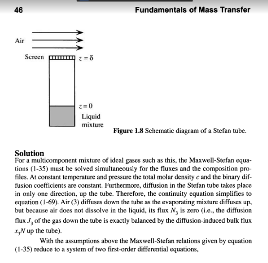
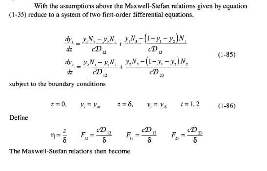
Example 1.17 Multicomponent, Steady-State, Gaseous Diffusion in a Stefan Tube (Taylor and Krishna, 1993) The Stefan tube, depicted schematically in Figure 1.8, is a simple device sometimes used for measuring diffusion coefficients in binary vapor mixtures. In the bottom of the tube is a pool of quiescent liquid. The vapor that evaporates from this pool diffus- es to the top of the tube. A stream of gas across the top of the tube keeps the mole frac- tion of the diffusing vapors there to essentially zero. The compositon of the vapor at the vapor-liquid interface is its equilibrium value. Carty and Schrodt (1975) evapo- rated a binary liquid mixture of acetone (1) and methanol (2) in a Stefan tube. Air (3) was used as the carrier gas. In one of their experiments the composition of the vapor at the liquid interface was y, = 0.319, y2 = 0.528, and yz = 0.153. The pressure and temperature in the gas phase were 99.4 kPa and 328.5 K, respectively. The length of the diffusion path was 0.24 m. The MS diffusion coefficients of the three binary pairs are: D. = 8.48 mm/s D,=13.72 mmIs D,=19.91 mm's Calculate the molar fluxes of acetone and methanol, and the composition profiles pre- dicted by the Maxwell-Stefan equations. Compare your results with the experimental data. 46 Fundamentals of Mass Transfer Air Screen 8 z = 0 Liquid mixture Figure 1.8 Schematic diagram of a Stefan tube. Solution For a multicomponent mixture of ideal gases such as this, the Maxwell-Stefan equa- tions (1-35) must be solved simultaneously for the fluxes and the composition pro- files. At constant temperature and pressure the total molar density c and the binary dif- fusion coefficients are constant. Furthermore, diffusion in the Stefan tube takes place in only one direction, up the tube. Therefore, the continuity equation simplifies to equation (1-69). Air (3) diffuses down the tube as the evaporating mixture diffuses up, but because air does not dissolve in the liquid, its flux N, is zero (i.e., the diffusion flux Jg of the gas down the tube is exactly balanced by the diffusion-induced bulk flux x N up the tube). With the assumptions above the Maxwell-Stefan relations given by equation (1-35) reduce to a system of two first-order differential equations, With the assumptions above the Maxwell-Stefan relations given by equation (1-35) reduce to a system of two first-order differential equations, dz (1-85) dy, y,N, - y,N, VN, -(1- y, - y,)N, D. CD dy, - y,N, - y, N, , ,N,-(1-y; - y)N, y1. dz subject to the boundary conditions D2