On the attached summarize what you read in the first section after you see the equations in (15.9).

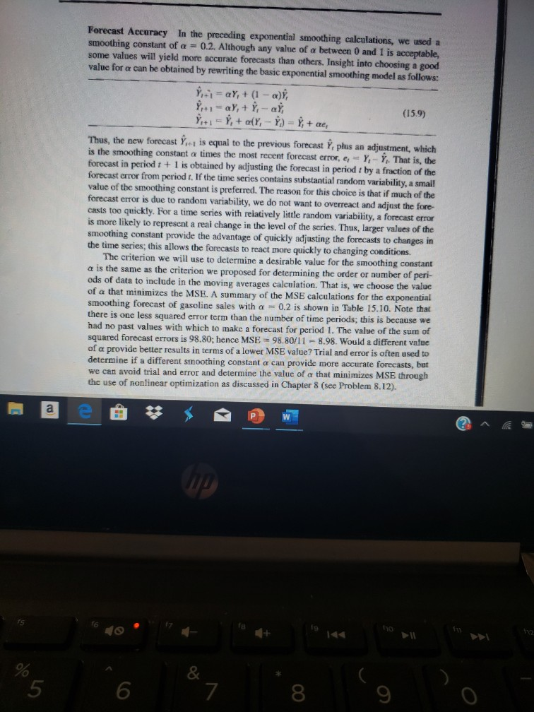
Forecast Accuracy in the preceding exponential smoothing calculations, we used a smoothing constant of a = 0.2. Although any value of a between 0 and 1 is acceptable, some values will yield more accurate forecasts than others. Insight into choosing a good value for a can be obtained by rewriting the basic exponential smoothing model as follows: 9-1 aY, + (1 - a), aY,+ - ah (15.9) Y+1 = Y, + a(Y, - Y) = Y, +ae, Thus, the new forecast Y - is equal to the previous forecast Y, plus an adjustment, which is the smoothing constant a times the most recent forecast error, e Y-Y. That is, the forecast in period 1 + 1 is obtained by adjusting the forecast in period / by a fraction of the forecast error from period t. If the time series contains substantial random variability, a small value of the smoothing constant is preferred. The reason for this choice is that if much of the is due to random variability, we do not want to overreact and adjust the fore casts too quickly. For a time series with relatively little random variability, a forecast error is more likely to represent a real change in the level of the series. Thus, larger values of the smoothing constant provide the advantage of quickly adjusting the forecasts to changes in the time series, this allows the forecasts to react more quickly to changing conditions The criterion we will use to determine a desirable value for the smoothing constant a is the same as the criterion we proposed for determining the order or number of peri- ods of data to include in the moving averages calculation. That is, we choose the value of a that minimizes the MSE. A summary of the MSE calculations for the exponential smoothing forecast of gasoline sales with a 0.2 is shown in Table 15.10. Note that there is one less squared error term than the number of time periods, this is because we had no past values with which to make a forecast for period 1. The value of the sum of squared forecast errors is 98.80; hence MSE 98.80/11 -8.98. Would a different value of a provide better results in terms of a lower MSE value? Trial and error is often used to determine if a different smoothing constant a can provide more accurate forecasts, but we can avoid trial and error and determine the value of a that minimizes MSE through the use of nonlinear optimization as discussed in Chapter 8 (see Problem 8.12). 5 lo 5 7 8