Only answer.......
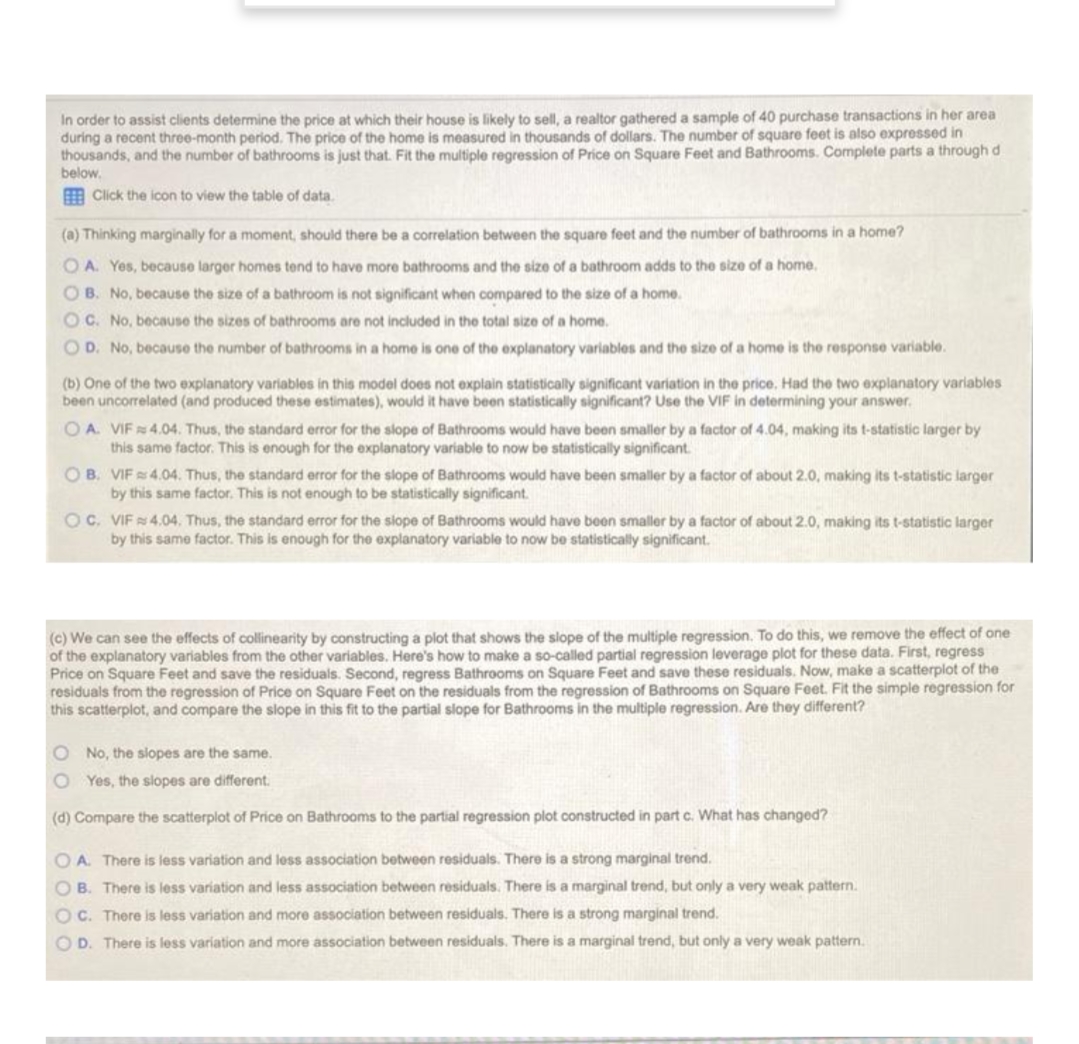
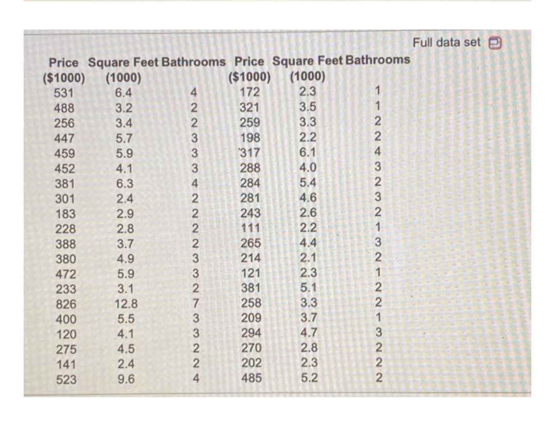
In order to assist clients determine the price at which their house is likely to sell, a realtor gathered a sample of 40 purchase transactions in her area during a recent three-month period. The price of the home is measured in thousands of dollars. The number of square feet is also expressed in thousands, and the number of bathrooms is just that. Fit the multiple regression of Price on Square Feet and Bathrooms. Complete parts a through d below. Click the icon to view the table of data. (a) Thinking marginally for a moment, should there be a correlation between the square feet and the number of bathrooms in a home? O A. Yes, because larger homes tend to have more bathrooms and the size of a bathroom adds to the size of a home. O B. No, because the size of a bathroom is not significant when compared to the size of a home. C. No, because the sizes of bathrooms are not included in the total size of a home. D. No, because the number of bathrooms in a home is one of the explanatory variables and the size of a home is the response variable (b) One of the two explanatory variables in this model does not explain statistically significant variation in the price, Had the two explanatory variables been uncorrelated (and produced these estimates), would it have been statistically significant? Use the VIF in determining your answer. O A. VIF 4.04. Thus, the standard error for the slope of Bathrooms would have been smaller by a factor of 4.04, making its t-statistic larger by this same factor. This is enough for the explanatory variable to now be statistically significant. O B. VIF # 4.04. Thus, the standard error for the slope of Bathrooms would have been smaller by a factor of about 2.0, making its t-statistic larger by this same factor. This is not enough to be statistically significant. C. VIF # 4.04, Thus, the standard error for the slope of Bathrooms would have been smaller by a factor of about 2.0, making its t-statistic larger by this same factor. This is enough for the explanatory variable to now be statistically significant. (c) We can see the effects of collinearity by constructing a plot that shows the slope of the multiple regression, To do this, we remove the effect of one of the explanatory variables from the other variables. Here's how to make a so-called partial regression leverage plot for these data. First, regress Price on Square Feet and save the residuals. Second, regress Bathrooms on Square Feet and save these residuals. Now, make a scatterplot of the residuals from the regression of Price on Square Feet on the residuals from the regression of Bathrooms on Square Feet. Fit the simple regression for this scatterplot, and compare the slope in this fit to the partial slope for Bathrooms in the multiple regression. Are they different? No, the slopes are the same. Yes, the slopes are different. (d) Compare the scatterplot of Price on Bathrooms to the partial regression plot constructed in part c. What has changed? O A. There is less variation and less association between residuals. There is a strong marginal trend. O B. There is less variation and less association between residuals. There is a marginal trend, but only a very weak pattern. O C. There is less variation and more association between residuals. There is a strong marginal trend. O D. There is less variation and more association between residuals. There is a marginal trend, but only a very weak pattern.Full data set Price Square Feet Bathrooms Price Square Feet Bathrooms ($1000) (1000) ($1000) (1000) 531 6.4 172 2.3 488 3.2 321 3.5 256 3.4 259 3.3 447 5.7 198 2.2 459 5.9 317 6.1 452 4.1 288 4.0 381 6.3 284 5.4 301 2.4 281 4.6 183 2.9 243 2.6 228 2.8 111 2.2 A N N W W N N W W N N N N A W WONNA 388 3.7 N N N W - N N - NW - NONWANN- - 265 4.4 380 4.9 214 2.1 472 5.9 121 2.3 233 3.1 381 5.1 826 12.8 258 3.3 400 5.5 209 3.7 120 4.1 294 4.7 275 4.5 270 2.8 141 2.4 202 2.3 523 9.6 485 5.2


